A comprehensive time-series benchmark evaluating state-of-the-art deep learning architectures (PatchTST, TFT, N-HiTS) against traditional gradient boosting (CatBoost) for accurate 24-hour load prediction.
Implementations of IQL, QMIX, VDN, COMA, QTRAN, MAVEN, CommNet, DyMA-CL, and G2ANet on SMAC, the decentralised micromanagement scenario of StarCraft II
A Modular Framework for 3D Gaussian Splatting and Beyond
关键参数与规格
关键参数与规格
参数
值
语言
Python
类别
Model Development
子类别
Architecture
星标数
1,769
分叉数
302
贡献者
6
创建日期
2016-09-16
更新日期
2026-10-08
1 天星标数
0
7 天星标数
0
排名
9,529
上次排名
9,565
排名变化
36
7 天星标排名
12,331
上次 7 天星标排名
9,681
7 天星标排名变化
-2,650
总星标排名
7,052
上次总星标排名
7,044
总星标排名变化
-8
国家
UK
README 摘录
Fast Wavenet: An efficient Wavenet generation implementation Our implementation speeds up Wavenet generation by eliminating redundant convolution operations. A naive implementation of Wavenet generation is O(2^L), while ours is O(L), where L is the number of layers. While other Wavenet repos focus on training on a large corpus of data and generating samples, ours mostly describes an efficient generation algorithm (which is super simple), and provides an example implementation. We note that while not explicitly stated in
the Wavenet paper, we talked to the authors, and they are doing something similar. For more about Wavenet, see DeepMind's blog post. If you find this work useful and use it on your own research, please cite our paper. Timing experiments We generated from a model with 2 blocks of L layers each, using a naive implementation and ours. When L is small the naive implementation performs better than expected due to GPU parallelization of the convolution operations. But when
L is large, the efficient implementation really shines. General purpose While this algorithm works well for auto-regressive models like Wavenet, it would be useful anytime you need to run a causal dilated convolutional neural network fast. For instance: classification/regression on streaming data. Though these ideas generalize to larger filter sizes. During generation, the computational graph used to compute a single output value can be seen as a binary tree. The input nodes (blue) are the leaves of the
tree, and the output is the root. The intermediate computations are the red nodes. The edges of the graph correspond to matrix multiplies. Since the computation is a binary tree, the overall computation time for graph is O(2^L). However, since this model is being applied repeatedly over time, there is a lot of redundant computation, which we can cache to increase the speed of generating a single sample. The key insight is this: given certain nodes in the
graph, we have all the information we need to compute the current output. We call these nodes the **recurrent states** in analogy to RNNs. These nodes have already been computed, all we need to do is cache them. Note that at the next time point, we will need a different subset of recurrent states. As a result we need to cache several **recurrent states** per layer. The number we need to keep is equal to the **dilation** of that layer
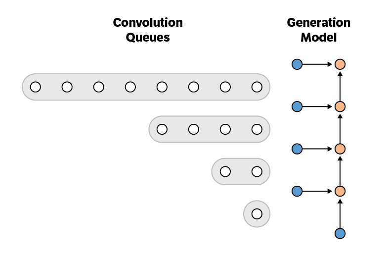
. Algorithm components The algorithm has two components: **Generation Model** **Convolution Queues** The generation model can be viewed as 1 step of a recurrent neural network. It takes as input: the current observation and several recurrent states, and computes: the output prediction and new recurrent states. The convolution queues store the new recurrent states which have been computed by the layer below. Algorithm Initialize the **generation model** with the weights from the pre-trained convolutional network. For each layer, initialize the
**convolution queue**. The max length of the queue equals the dilation of that layer. Repeat: Pop phase Push phase **Pop
常见问题
记录了多少星标和分叉?
tomlepaine/fast-wavenet 有 1,769 个星标和 302 个分叉。
仓库排名是多少?
tomlepaine/fast-wavenet 排名第 9,529。
记录的语言和类别是什么?
tomlepaine/fast-wavenet 有 1,769 个星标,语言为 Python,类别为 Model Development。
Fast Wavenet: An efficient Wavenet generation implementation

Our implementation speeds up Wavenet generation by eliminating redundant convolution operations. A naive implementation of Wavenet generation is O(2^L), while ours is O(L), where L is the number of layers.
While other Wavenet repos focus on training on a large corpus of data and generating samples, ours mostly describes an efficient generation algorithm (which is super simple), and provides an example implementation.
We note that while not explicitly stated in the Wavenet paper, we talked to the authors, and they are doing something similar.
If you find this work useful and use it on your own research, please cite our paper.
@article{paine2016fast,
  title={Fast Wavenet Generation Algorithm},
  author={Paine, Tom Le and Khorrami, Pooya and Chang, Shiyu and Zhang, Yang and Ramachandran, Prajit and Hasegawa-Johnson, Mark A and Huang, Thomas S},
  journal={arXiv preprint arXiv:1611.09482},
  year={2016}
}
Timing experiments

We generated from a model with 2 blocks of L layers each, using a naive implementation and ours. Results are averaged over 100 repeats. When L is small the naive implementation performs better than expected due to GPU parallelization of the convolution operations. But when L is large, the efficient implementation really shines.
General purpose
While this algorithm works well for auto-regressive models like Wavenet, it would be useful anytime you need to run a causal dilated convolutional neural network fast. For instance: classification/regression on streaming data.
Here we focus on generation for dilated causal convolution networks (E.g. Wavenet) with filter size 2. Though these ideas generalize to larger filter sizes.
During generation, the computational graph used to compute a single output value can be seen as a binary tree.

The input nodes (blue) are the leaves of the tree, and the output is the root. The intermediate computations are the red nodes. The edges of the graph correspond to matrix multiplies. Since the computation is a binary tree, the overall computation time for graph is O(2^L). When L is large, this is horrible.
However, since this model is being applied repeatedly over time, there is a lot of redundant computation, which we can cache to increase the speed of generating a single sample.
The key insight is this: given certain nodes in the graph, we have all the information we need to compute the current output. We call these nodes the recurrent states in analogy to RNNs. These nodes have already been computed, all we need to do is cache them.

Note that at the next time point, we will need a different subset of recurrent states. As a result we need to cache several recurrent states per layer. The number we need to keep is equal to the dilation of that layer.

Algorithm components
The algorithm has two components:
Generation Model
Convolution Queues
The generation model can be viewed as 1 step of a recurrent neural network. It takes as input: the current observation and several recurrent states, and computes: the output prediction and new recurrent states.
The convolution queues store the new recurrent states which have been computed by the layer below.
Algorithm
Initialize the generation model with the weights from the pre-trained convolutional network.
For each layer, initialize the convolution queue. The max length of the queue equals the dilation of that layer. Fill it with zero recurrent states. (See above).
Repeat:
Pop phase
Push phase
Pop phase: For each convolution queue pop the recurrent state and feed it to the corresponding state of the generation model, then calculate the new hidden states and output.

Push phase: For each new hidden state push it into the convolution queue of the layer above.