neurodiffeq

Citation

A 2nd NeuroDiffEq paper has been published. Please make sure to cite both if you have been using features that became available after the 2020 version.

@article{chen2020neurodiffeq,
  title={NeuroDiffEq: A Python package for solving differential equations with neural networks},
  author={Chen, Feiyu and Sondak, David and Protopapas, Pavlos and Mattheakis, Marios and Liu, Shuheng and Agarwal, Devansh and Di Giovanni, Marco},
  journal={Journal of Open Source Software},
  volume={5},
  number={46},
  pages={1931},
  year={2020}
}

@article{liu2025recent,
  title={Recent Advances of NeuroDiffEq--An Open-Source Library for Physics-Informed Neural Networks},
  author={Liu, Shuheng and Protopapas, Pavlos and Sondak, David and Chen, Feiyu},
  journal={arXiv preprint arXiv:2502.12177},
  year={2025}
}

🔥🔥🔥Did you know that neurodiffeq supports solution bundles and can be used to solve reverse problems? See here!

:mortar_board: Already familiar with neurodiffeq? :point_down: Jump to FAQs.

Introduction

neurodiffeq is a package for solving differential equations with neural networks. Differential equations are equations that relate some function with its derivatives. They emerge in various scientific and engineering domains. Traditionally these problems can be solved by numerical methods (e.g. finite difference, finite element). While these methods are effective and adequate, their expressibility is limited by their function representation. It would be interesting if we can compute solutions for differential equations that are continuous and differentiable.

As universal function approximators, artificial neural networks have been shown to have the potential to solve ordinary differential equations (ODEs) and partial differential equations (PDEs) with certain initial/boundary conditions. The aim of neurodiffeq is to implement these existing techniques of using ANN to solve differential equations in a way that allow the software to be flexible enough to work on a wide range of user-defined problems.

Installation

Using pip

Like most standard libraries, neurodiffeq is hosted on PyPI. To install the latest stable relesase,

pip install -U neurodiffeq  # '-U' means update to latest version

Manually

Alternatively, you can install the library manually to get early access to our new features. This is the recommended way for developers who want to contribute to the library.

git clone https://github.com/NeuroDiffGym/neurodiffeq.git
cd neurodiffeq && pip install -r requirements
pip install .  # To make changes to the library, use `pip install -e .`
pytest tests/  # Run tests. Optional.

Getting Started

We are happy to help you with any questions. In the meantime, you can checkout the FAQs.

To view complete tutorials and documentation of neurodiffeq, please check Official Documentation.

In addition to the documentations, we have recently made a quick walkthrough Demo Video with slides.

Example Usages

Imports

from neurodiffeq import diff
from neurodiffeq.solvers import Solver1D, Solver2D
from neurodiffeq.conditions import IVP, DirichletBVP2D
from neurodiffeq.networks import FCNN, SinActv

ODE System Example

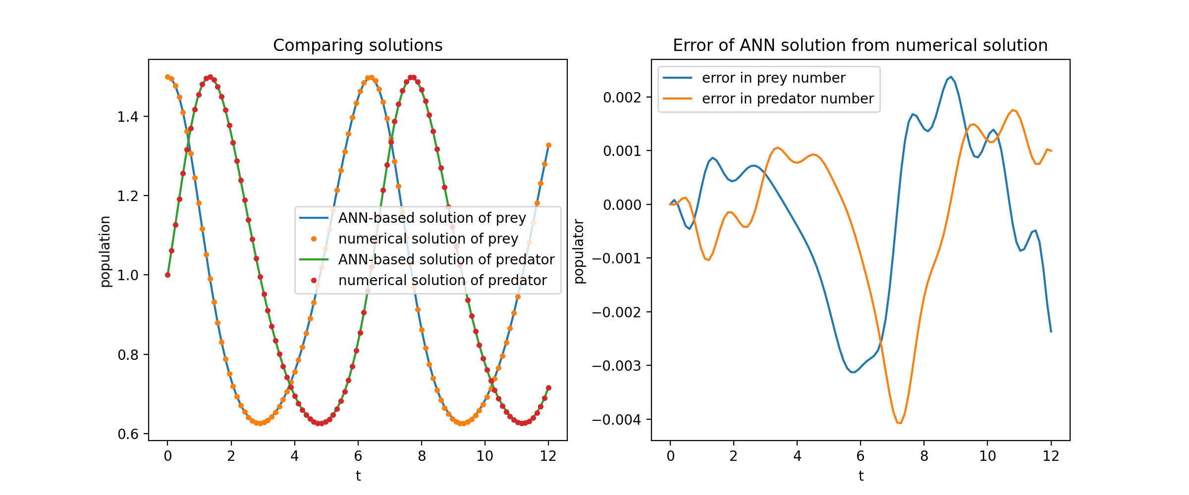
Here we solve a non-linear system of two ODEs, known as the Lotka–Volterra equations. There are two unknown functions (u and v) and a single independent variable (t).

def ode_system(u, v, t): 
    return [diff(u,t)-(u-u*v), diff(v,t)-(u*v-v)]

conditions = [IVP(t_0=0.0, u_0=1.5), IVP(t_0=0.0, u_0=1.0)]
nets = [FCNN(actv=SinActv), FCNN(actv=SinActv)]

solver = Solver1D(ode_system, conditions, t_min=0.1, t_max=12.0, nets=nets)
solver.fit(max_epochs=3000)
solution = solver.get_solution()

solution is a callable object, you can pass in numpy arrays or torch tensors to it like

u, v = solution(t, to_numpy=True)  # t can be np.ndarray or torch.Tensor

Plotting u and v against their analytical solutions yields something like:

PDE System Example

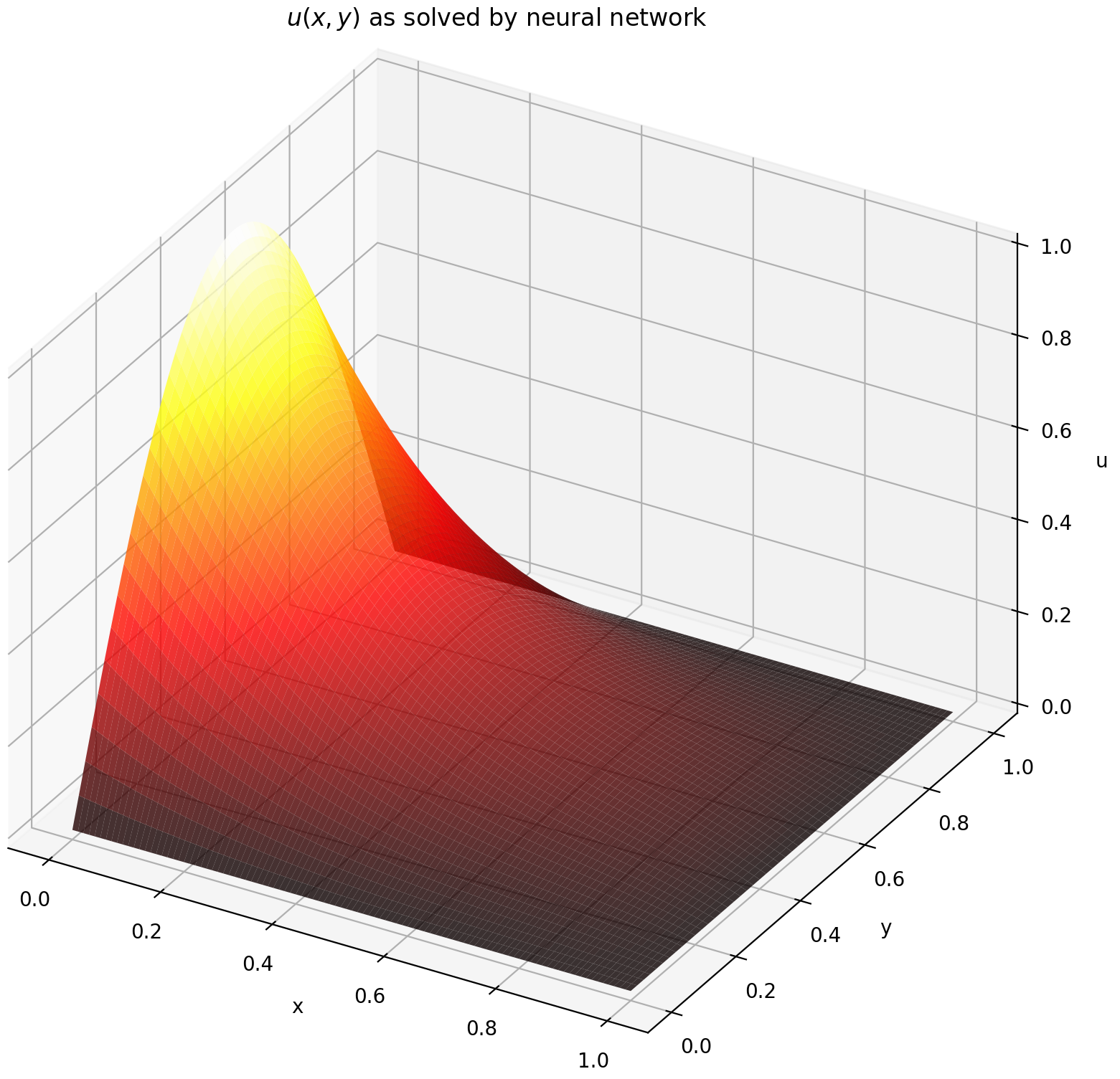
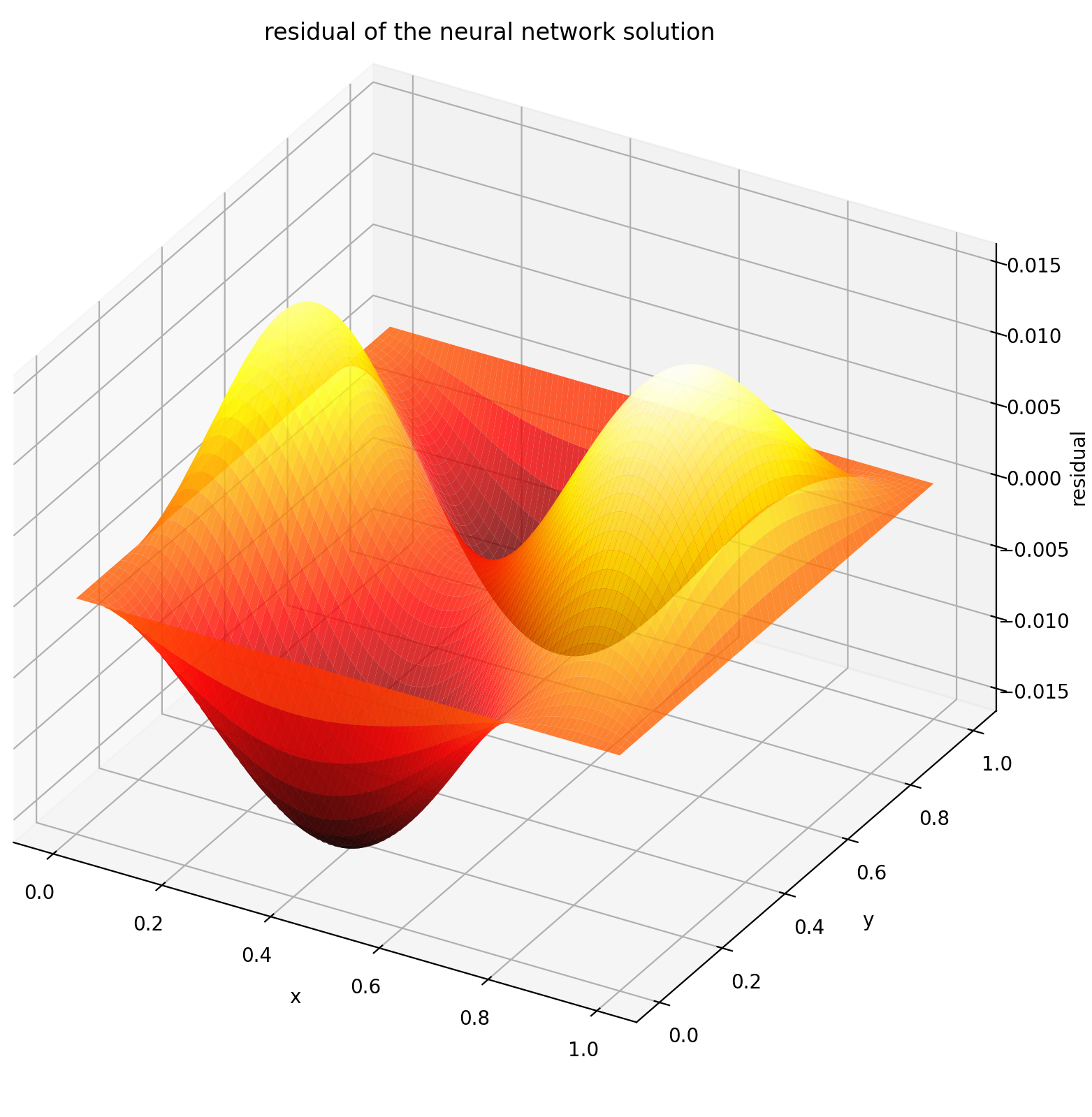
Here we solve a Laplace Equation with Dirichlet boundary conditions on a rectangle. Note that we choose Laplace equation for its simplicity of computing analytical solution. In practice, you can attempt any nonlinear, chaotic PDEs, provided you tune the solver well enough.

Solving a 2-D PDE system is quite similar to solving ODEs, except there are two variables x and y for boundary value problems or x and t for initial boundary value problems, both of which are supported.

def pde_system(u, x, y):
    return [diff(u, x, order=2) + diff(u, y, order=2)]

conditions = [
    DirichletBVP2D(
        x_min=0, x_min_val=lambda y: torch.sin(np.pi*y),
        x_max=1, x_max_val=lambda y: 0,                   
        y_min=0, y_min_val=lambda x: 0,                   
        y_max=1, y_max_val=lambda x: 0,                   
    )
]
nets = [FCNN(n_input_units=2, n_output_units=1, hidden_units=(512,))]

solver = Solver2D(pde_system, conditions, xy_min=(0, 0), xy_max=(1, 1), nets=nets)
solver.fit(max_epochs=2000)
solution = solver.get_solution()

The signature of solution for a 2D PDE is slightly different from that of an ODE. Again, it takes in either numpy arrays or torch tensors.

u = solution(x, y, to_numpy=True)

Evaluating u on [0,1] × [0,1] yields the following plots

ANN-Based Solution	Residual of PDE

Using a Monitor

A monitor is a tool for visualizing PDE/ODE solutions as well as history of loss and custom metrics during training. Jupyter Notebooks users need to run the %matplotlib notebook magic. For Jupyter Lab users, try %matplotlib widget.

from neurodiffeq.monitors import Monitor1D
...
monitor = Monitor1D(t_min=0.0, t_max=12.0, check_every=100)
solver.fit(..., callbacks=[monitor.to_callback()])

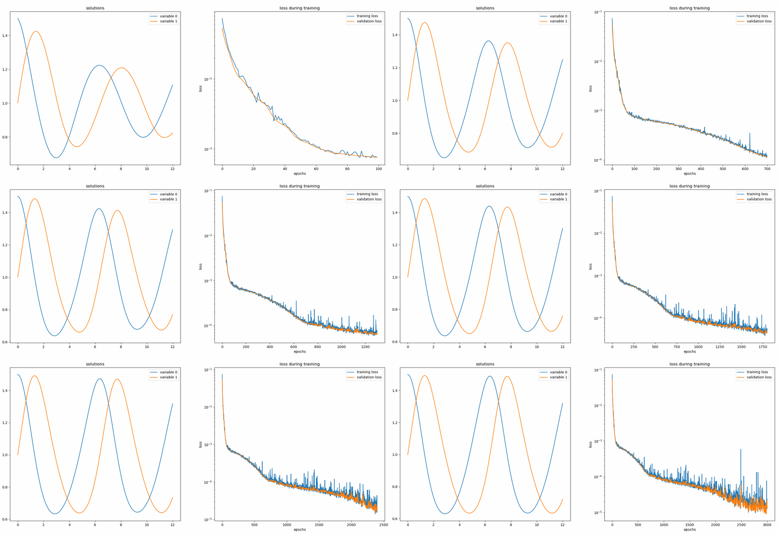
You should see the plots update every 100 epoch as well as on the last epoch, showing two plots — one for solution visualization on the interval [0,12] and the other for loss history (training and validation).

Custom Networks

For convenience, we have implemented an FCNN – fully-connected neural network, whose hidden units and activation functions can be customized.

from neurodiffeq.networks import FCNN
# Default: n_input_units=1, n_output_units=1, hidden_units=[32, 32], activation=torch.nn.Tanh
net1 = FCNN(n_input_units=..., n_output_units=..., hidden_units=[..., ..., ...], activation=...) 
...
nets = [net1, net2, ...]

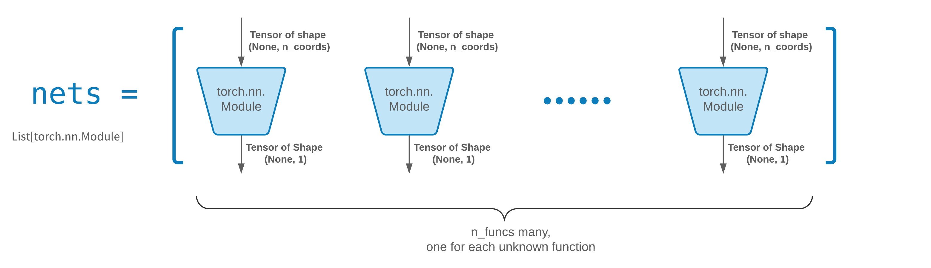
FCNN is usually a good starting point. For advanced users, solvers are compatible with any custom torch.nn.Module. The only constraints are:

1. The modules takes in a tensor of shape (None, n_coords) and the outputs a tensor of shape (None, 1).

2. There must be a total of n_funcs modules in nets to be passed to solver = Solver(..., nets=nets).

Acutally, neurodiffeq has a single_net feature that doesn't obey the above rules, which won't be covered here.

Read the PyTorch tutorial on building your own network (a.k.a module) architecture.

Transfer Learning

Transfer learning is easily done by serializing old_solver.nets (a list of torch modules) to disk and then loading them and passing to a new solver:

old_solver.fit(max_epochs=...)
# ... dump `old_solver.nets` to disk

# ... load the networks from disk, store them in some `loaded_nets` variable
new_solver = Solver(..., nets=loaded_nets)
new_solver.fit(max_epochs=...)

We currently working on wrapper functions to save/load networks and other internal variables of Solvers. In the meantime, you can read the PyTorch tutorial on saving and loading your networks.

Sampling Strategies

In neurodiffeq, the networks are trained by minimizing loss (ODE/PDE residuals) evaluated on a set of points in the domain. The points are randonly resampled every time. To control the number, distribution, and bounding domain of sampled points, you can specify your own training/valiadation generators.

from neurodiffeq.generators import Generator1D

# Default t_min=0.0, t_max=1.0, method='uniform', noise_std=None
g1 = Generator1D(size=..., t_min=..., t_max=..., method=..., noise_std=...)
g2 = Generator1D(size=..., t_min=..., t_max=..., method=..., noise_std=...)

solver = Solver1D(..., train_generator=g1, valid_generator=g2)

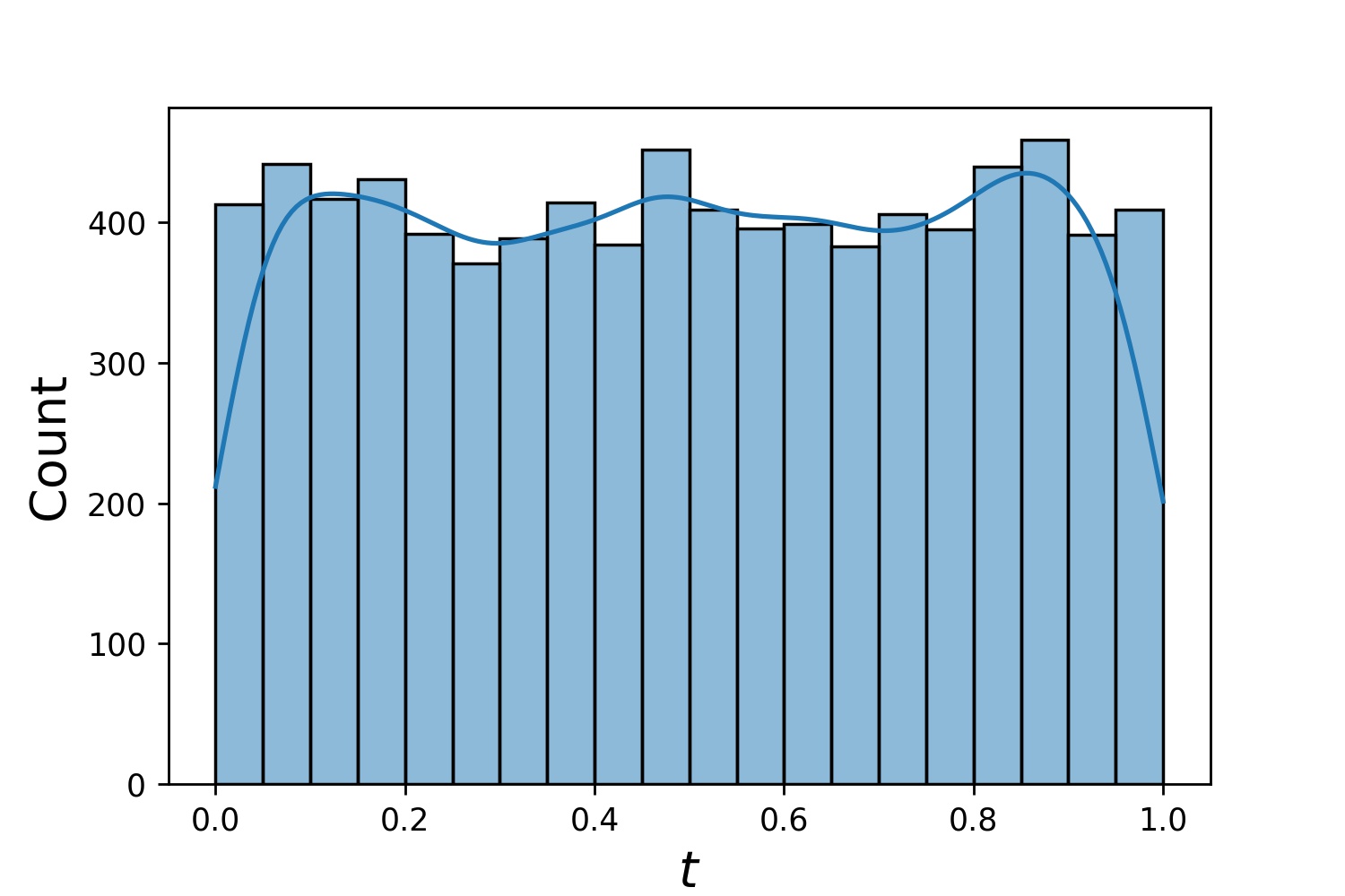
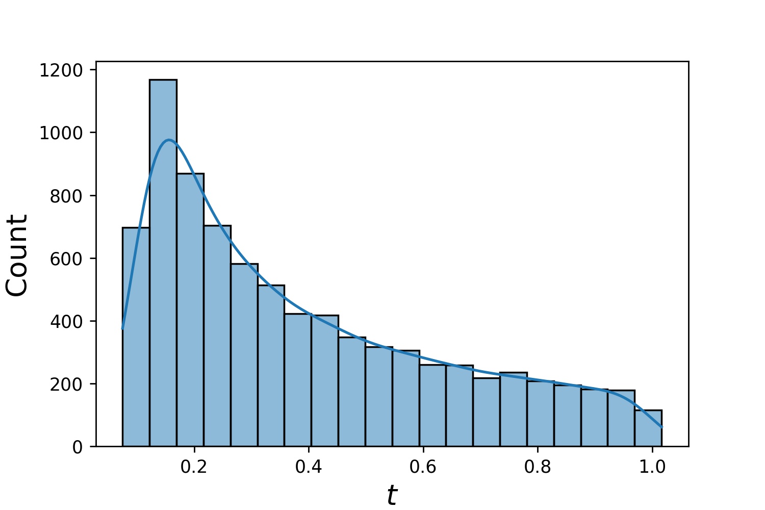
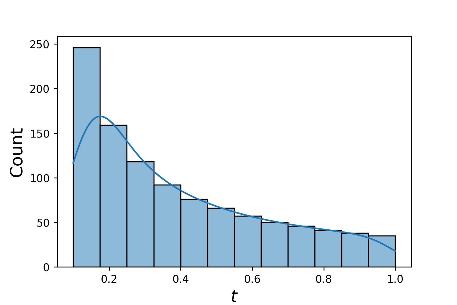
Here are some sample distributions of a Generator1D.

Generator1D(8192, 0.0, 1.0, method='uniform')	Generator1D(8192, -1.0, 0.0, method='log-spaced-noisy', noise_std=1e-3)

Note that when both train_generator and valid_generator are specified, t_min and t_max can be omitted in Solver1D(...). In fact, even if you pass t_min, t_max, train_generator, valid_generator together, the t_min and t_max will still be ignored.

Combining Generators

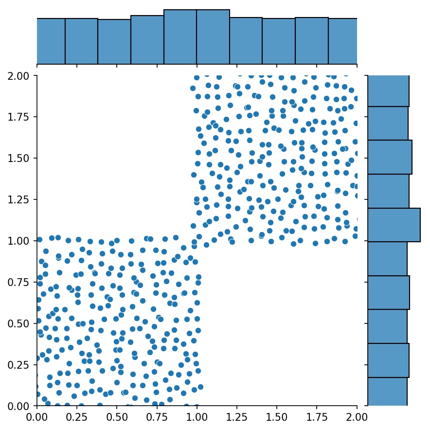
Another nice feature of the generators is that you can concatenate them, for example

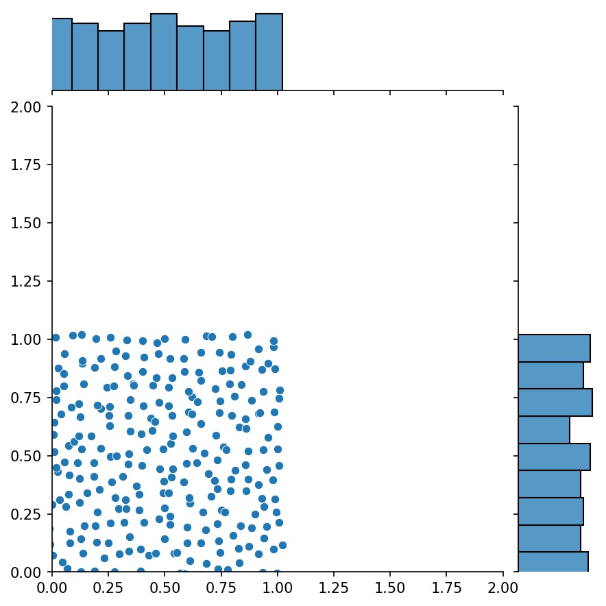
g1 = Generator2D((16, 16), xy_min=(0, 0), xy_max=(1, 1))
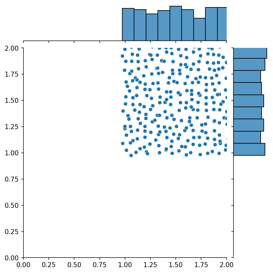
g2 = Generator2D((16, 16), xy_min=(1, 1), xy_max=(2, 2))
g = g1 + g2

Here, g will be a generator that outputs the combined samples of g1 and g2

g1	g2	g1 + g2

Sampling Higher Dimensions

You can use Generator2D, Generator3D, etc. for sampling points in higher dimensions. But there's also another way

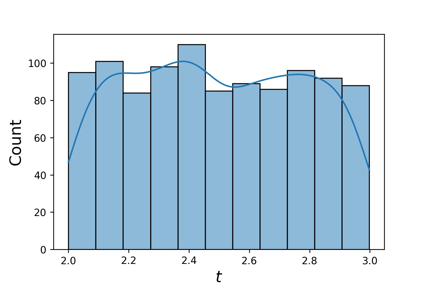
g1 = Generator1D(1024, 2.0, 3.0, method='uniform')
g2 = Generator1D(1024, 0.1, 1.0, method='log-spaced-noisy', noise_std=0.001)
g = g1 * g2

Here, g will be a generator which yields 1024 points in a 2-D rectangle (2,3) × (0.1,1) every time. The x-coordinates of them are drawn from (2,3) using strategy uniform and the y-coordinate drawn from (0.1,1) using strategy log-spaced-noisy.

g1	g2	g1 * g2

Solution Bundle and Reverse Problems

Sometimes, it is interesting to solve a bundle of equations at once. For example, you may want to solve differential equations of the form du/dt + λu = 0 under the initial condition u(0) = U0. You may want to solve this for all λ and U0 at once, by treating them as inputs to the neural networks.

One such application is for chemical reactions, where the reaction rate is unknown. Different reaction rates correspond to different solutions, and only one solution matches observed data points. You maybe interested in first solving for a bundle of solutions, and then determining the best reaction rates (aka equation parameters). The second step is known as the inverse problem.

Here's an example of how to do this using neurodiffeq:

1. Let's say we have an equation du/dt + λu = 0 and initial condition u(0) = U0 where λ and U0 are unknown constants. We also have a set of observations t_obs and u_obs. We first import BundleSolver and BundleIVP which is necessary to obtaining a solution bundle:

   from neurodiffeq.conditions import BundleIVP
   from neurodiffeq.solvers import BundleSolver1D
   
   import matplotlib.pyplot as plt
   import numpy as np
   import torch
   from neurodiffeq import diff
   

2. We determine the domain of input t, as well as the domain of parameters λ and U0. We also need to make a decision of the order of the parameters. Namely, which should be the first parameter, and which should be the second. For the purpose of this demo, we choose λ to be the first parameter (index 0), and U0 to be the second (index 1). It is very important to keep track of the indices of the parameters.

   T_MIN, T_MAX = 0, 1
   LAMBDA_MIN, LAMBDA_MAX = 3, 5  # first parameter,  index = 0
   U0_MIN, U0_MAX = 0.2, 0.6       # second parameter, index = 1
   

3. We then define the conditions and solver as usual, except that we use BundleIVP and BundleSolver1D instead of IVP and Solver1D. The interface of these two is very similar to IVP and Solver1D. You can find out more in the API reference.

   # equation parameters comes after inputs (usually temporal and spatial coordinates)
   diff_eq = lambda u, t, lmd: [diff(u, t) + lmd * u]
   
   # The keyword argument must be named "u_0" in BundleIVP. If you use anything else, e.g. `y0`, `u0`, etc., it won't work.
   conditions = [
       BundleIVP(t_0=0, u_0=None, bundle_param_lookup={'u_0': 1})  # u_0 has index 1
   ]
   
   solver = BundleSolver1D(
       ode_system=diff_eq,
       conditions=conditions,
       t_min=T_MIN, t_max=T_MAX, 
       theta_min=[LAMBDA_MIN, U0_MIN],  # λ has index 0; u_0 has index 1
       theta_max=[LAMBDA_MAX, U0_MAX],  # λ has index 0; u_0 has index 1
       eq_param_index=(0,),             # λ is the only equation parameter, which has index 0
       n_batches_valid=1,
   )
   

   Since λ is a parameter in the equation and U0 is a parameter in the initial condition, we must include λ in the diff_eq and U0 in the condition. If a parameter is present in both the equation and the condition, it must be included in both places. All elements of conditions passed to BundleSovler1D must be Bundle* conditions, even if they don't have parameters.

4. Now, we can train it and obtain the solution as we normally would.

   solver.fit(max_epochs=1000)
   solution = solver.get_solution(best=True)
   

   The solution expects three inputs - t, λ and U0. All inputs must have the same shape. For example, if you are interested in fixing λ=4 and U0=0.4 and plotting the solution u against t ∈ [0,1] , you can do the following

   t = np.linspace(0, 1)
   lmd = 4 * np.ones_like(t)
   u0 = 0.4 * np.ones_like(t)
   
   u = solution(t, lmd, u0, to_numpy=True)
   
   import matplotlib.pyplot as plt
   plt.plot(t, u)
   

5. Once you have a bundled solution, you can find a set of parameters (λ, U0) that matches observed data points (t_i, u_i) most closely. This is achieved using simple gradient descent. In the following toy example, we assume there are only three data points u(0.2) = 0.273, u(0.5)=0.129, and u(0.8) = 0.0609. The following is classical PyTorch workflow.

   # observed data points
   t_obs = torch.tensor([0.2, 0.5, 0.8]).reshape(-1, 1)
   u_obs = torch.tensor([0.273, 0.129, 0.0609]).reshape(-1, 1)
   
   # random intialization of λ and U0; keep track of their gradient
   lmd_tensor = torch.rand(1) * (LAMBDA_MAX - LAMBDA_MIN) + LAMBDA_MIN
   u0_tensor = torch.rand(1) * (U0_MAX - U0_MIN) + U0_MIN
   adam = torch.optim.Adam([lmd_tensor.requires_grad_(True), u0_tensor.requires_grad_(True)], lr=1e-2)
   
   # run gradient descent for 10000 epochs
   for _ in range(10000):
       output = solution(t_obs, lmd_tensor * torch.ones_like(t_obs), u0_tensor * torch.ones_like(t_obs))
       loss = ((output - u_obs) ** 2).mean()
       loss.backward()
       adam.step()
       adam.zero_grad()
      
   print(f"λ = {lmd_tensor.item()}, U0={u0_tensor.item()}, loss = {loss.item()}")
   

FAQ

Q: How to use GPU for training?

Simple. When importing neurodiffeq, the library automatically detects if CUDA is available on your machine. Since the library is based on PyTorch, it will set default tensor type to torch.cuda.DoubleTensor for if a compatible GPU device is found.

Q: How to use pretrained nets?

Refer to Sections Custom Networks and Transfer Learning.

Q: How to change the learning rate?

The standard PyTorch way.

1. Build your networks as explained in Custom Networks: nets = [FCNN(), FCN(), ...]

2. Instantiate a custom optimizer and pass all parameters of these networks to it

   parameters = [p for net in nets for p in net.parameters()]  # list of paramters of all networks
   MY_LEARNING_RATE = 5e-3
   optimizer = torch.optim.Adam(parameters, lr=MY_LEARNING_RATE, ...)
   

3. Pass BOTH your nets and your optimizer to the solver: solver = Solver1D(..., nets=nets, optimizer=optimizer)

Q: I got a bad solution.

Unlike traditional numerial methods (FEM, FVM, etc.), the NN-based solution requires some hypertuning. The library offers the utmost flexibility to try any combination of hyperparameters.

• To use a different network architecture, you can pass in your custom torch.nn.Modules.
• To use a different optimizer, you can pass in your own optimizer to solver = Solver(..., optimizer=my_optim).
• To use a different sampling distribution, you can use built-in generators or write your own generators from scratch.
• To use a different sampling size, you can tweak the generators or change solver = Solver(..., n_batches_train).
• To dynamically change hyperparameters during training, checkout our callbacks feature.

Q: Any rules of thumbs?

• Don't use ReLU for activation, because its second-order derivative is identically 0.
• Re-scale your PDE/ODE in dimensionless form, preferably make everything range in [0,1]. Working with a domain like [0,1000000] is prone to failure because a) PyTorch initializes the modules weights to be relatively small and b) most activation functions (like Sigmoid, Tanh, Swish) are most nonlinear near 0.
• If your PDE/ODE is too complicated, consider trying curriculum learning. Start training your networks on a smaller domain, and then gradually expand until the whole domain is covered.

Contributing

Everyone is welcome to contribute to this project.

When contributing to this repository, we consider the following process:

1. Open an issue to discuss the change you are planning to make.
2. Go through Contribution Guidelines.
3. Make the change on a forked repository and update the README.md if changes are made to the interface.
4. Open a pull request.