Install Library

..with pip install -U git+https://github.com/emoen/Machine-Learning-for-Asset-Managers

from Machine_Learning_for_Asset_Managers import ch2_fitKDE_find_best_bandwidth as c import numpy as np c.findOptimalBWidth(np.asarray([21,3])) {'bandwidth': 10.0}

Machine-Learning-for-Asset-Managers

Implementation of code snippets and exercises from Machine Learning for Asset Managers (Elements in Quantitative Finance) written by Prof. Marcos López de Prado.

The project is for my own learning. If you want to use the consepts from the book - you should head over to Hudson & Thames. They have implemented these consepts and many more in mlfinlab.

For practical application see the repository: Machine-Learning-for-Asset-Managers-Oslo-Bors.

Note: In chapter 4 - there is a bug in the implementation of "Optimal Number of Clusters" algorithm (ONC) in the book (the code from the paper - DETECTION OF FALSE INVESTMENT STRATEGIES USING UNSUPERVISED LEARNING METHODS, de Prado and Lewis (2018) -
is different but is also incorrect ) https://quant.stackexchange.com/questions/60486/bug-found-in-optimal-number-of-clusters-algorithm-from-de-prado-and-lewis-201

The divide and conquer method of subspaces used by ONC can be problematic because if you embed a subspace into a space with a large eigen-value. The larger space can distort the clusters found in the subspace. ONC does precisely that - it embeds subspaces into the space consisting of the largest eigenvalues found in the correlation matrix. An outline describing the problem more rigorously can be found here: https://math.stackexchange.com/questions/4013808/metric-on-clustering-of-correlation-matrix-using-silhouette-score/4050616#4050616

Other clustering algorithms should be investigated like hierarchical clustering.

Chapter 2 Denoising and Detoning

Marcenko-Pasture theoretical probability density function, and empirical density function:

Figure 2.1:Marcenko-Pasture theoretical probability density function, and empirical density function:

Denoising a random matrix with signal using the constant residual eigenvalue method. This is done by fixing random eigenvalues. See code snippet 2.5

Figure 2.2: A comparison of eigenvalues before and after applying the residual eigenvalue method:

Detoned covariance matrix can be used to calculate minimum variance portfolio. The efficient frontier is the upper portion of the minimum variance frontier starting at the minimum variance portfolio. A denoised covariance matrix is less unstable to change.

Note: Excersize 2.7: "Extend function fitKDE in code snippet 2.2, so that it estimates through cross-validation the optimal value of bWidth (bandwidth)".

The script ch2_fitKDE_find_bandwidth.py implements this procedure and produces the (green) KDE in figure 2.3:

Figure 2.3: Calculated bandwidth(green line) together with histogram, and pdf. The green line is smoother. Bandwidth found: 0.03511191734215131

From code snippet 2.3 - with random matrix with signal: the histogram is how the eigenvalues of a random matrix with signal is distributed. Then the variance of the theoretical probability density function is calculated using the $fitKDE$ as the empirical probability density function. So finding a good value for bandwidth in fitKDE is needed to find the likeliest variance of the theoretical mp-pdf.

Figure 2.4: histogram and pdf of eigenvalues with signal

Chapter 3 Distance Metrics

• definition of a metric:
  1. identity of indiscernibles d(x,y) = 0 => x=y
  2. Symmetry d(x,y) = d(y,x)
  3. triangle inequality.
  • 1,2,3 => non-negativ, d(x,y) >= 0
• pearson correlation
• distance correlation
• angular distance
• Information-theoretic codependence/entropy dependence
  • cross-entropy: H[X] = - Σs ∈ SX p[x] log (p[x])
  • Kullback-Leilbler divergence: DKL[p||q] = - Σs ∈ SX p[x] log (q[x]/p[x]) = p[x] Σs ∈ S log (p[x]/q[x])
  • Cross-entropy: Hc[p||q] = H[x] = DKL[p||q]
  • Mutual information: Decrease in uncertainty in X from knowing Y: I[X,Y] = H[X] - H[X|Y] = H[X] + H[Y] - H[X,Y] = EX[DKL[p[y|x]||p[y]]]
  • variation of information: VI[X,Y] = H[X|Y] + H[Y|X] = H[X,Y] - I[X,Y]. It is uncertainty we expect in one variable given another variable: VI[X,Y] = 0 <=> X=Y
  • Kullback-Leilbler divergence is not a metric while variation of information is.

>>> ss.entropy([1./2,1./2], base=2)
1.0
>>> ss.entropy([1,0], base=2)
0.0
>>> ss.entropy([1./3,2./3], base=2)
0.9182958340544894

1. 1 bit of information in coin toss
2. 0 bit of information in deterministic outcome
3. less than 1 bit of information in unfair coin toss

• Angular distance: p_d = sqrt(1/2 - (1-rho(X, Y)))
• Absolute angular distance: p_d = sqrt(1/2 - (1-|rho|(X, Y)))
• Squared angular distance: p_d = sqrt(1/2 - (1-rho^2(X, Y)))

Standard angular distance is better used for long-only portfolio appliacations. Squared and Absolute Angular Distances for long-short portfolios.

Chapter 4 Optimal Clustering

Use unsupervised learning to maximize intragroup similarities and minimize intergroup similarities. Consider matrix X of shape N x F. N objects and F features. Features are used to compute proximity(correlation, mutual information) to N objects in an NxN matrix.

There are 2 types of clustering algorithms. Partitional and hierarchical:

1. Connectivity: hierarchical clustering
2. Centroids: like k-means
3. Distribution: gaussians
4. Density: search for connected dense regions like DBSCAN, OPTICS
5. Subspace: modeled on two dimension, feature and observation. Example

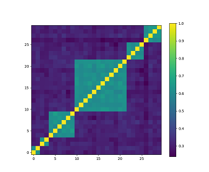
Generating of random block correlation matrices is used to simulate instruments with correlation. The utility for doing this is in code snippet 4.3, and it uses clustering algorithms optimal number of cluster (ONC) defined in snippet 4.1 and 4.2, which does not need a predefined number of clusters (unlike k-means), but uses an 'elbow method' to stop adding clusters. The optimal number of clusters are achieved when there is high intra-cluster correlation and low inter-cluster correlation. The silhouette score is used to minimize within-group distance and maximize between-group distance.

Random block correlation matrix. Light colors indicate a high correlation, and dark colors indicate a low correlation. In this example, the number of blocks K=6, minBlockSize=2, and number of instruments N=30
Applying the ONC algorithm to the random block correlation matrix. ONC finds all the clusters.

Chapter 5 Financial Labels

• Fixed-Horizon method
• Time-bar method
• Volume-bar method

Tiple-Barrier Method involves holding a position until

1. Unrealized profit target achieved
2. unrealized loss limit reached
3. Position is held beyond a maximum number of bars

Trend-scanning method: the idea is to identify trends and let them run for as long and as far as they may persists, without setting any barriers.

Example of trend-scanning labels on sine wave with gaussian noise:

trend-scanning with t-values which shows confidence in trend. 1 is high confidence going up and -1 is high confidence going down.

An alternative to look-forward algorithm as presented in the book is to use look-backward from the latest data-point to the window-size. E.g. if the latest data-point is at index 20 - and the window size is between 3 and 10 days. The look-backward algorithm will scan window at index 17 to 20 all the way back to index 11 to 20. Hence only considering the most recent information.

trend-scanning with t-values using look-backwards

Chapter 6 Feature Importance Analysis

"p-value does not measure the probability that neither the null nor the alternative hypothesis is true, or the significance of a result."

p-Values computed on a set of informative, redundant, and noisy explanatory variables. The explanatory variables has not the hightest p-values.

"Backtesting is not a research tool. Feature importance is." (Lopez de Prado) The Mean Decrease Impurity (MDI) algorithm deals with 3 out of 4 problems with p-values:

1. MDI is not imposing any tree structure, algebraic specification, or relying on any stochastic or distributional characteristics of the residuals (e.g. y=b0+b1*xi+ε)
2. betas are estimated from single sample, MDI relies on bootstrapping, so the variance can be reduced by the numbers of trees in the random forrest ensemble.
3. In MDI the goal is not to estimate a coefficient of a given algebraic equation (b_hat_0, b_hat_1) describing the probability of a null-hypotheses.
4. MDI does not correct of calculation in-sample, as there is no cross-validation.

MDI algorithm example

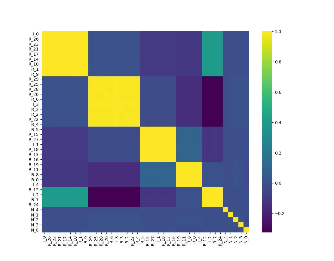
Figure 6.4 shows that ONC correctly recognizes that there are six relevant clusters(one cluster for each informative feature, plus one cluster of noise features), and it assigns the redundant features to the cluster that contains the informative feature from which the redundant features where derived. Given the low correlation across clusters, there is no need to replace the features with their residuals.

Next, apply the clustered MDI method to the clustered data:

Figure 6.5 Clustered MDI

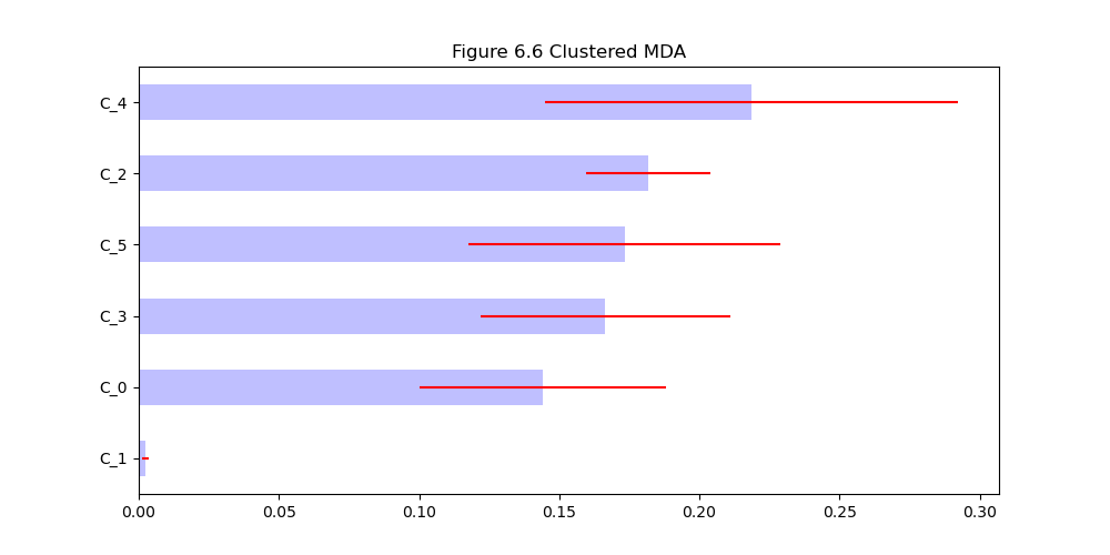
Clustered MDI works better han non-clustered MDI. Finally, apply the clustered MDA method to this data:

Figure 6.6 Clustered MDA

Conclusion: C_5 which is associated with noisy features is not important, and all other clusters has similar importance.

Chapter 7 Portfolio Construction

Convex portfolio optimization can calculate minimum variance portfolio and max sharp-ratio.

Definition Condition number: absolute value of the ratio between the maximum and minimum eigenvalues: A_n_n / A_m_m. The condition number says something about the instability of the instability caused by covariance structures. Definition trace = sum(diag(A)) - its the sum of the diagonal elements

Highly correlated time-series implies high condition number of the correlation matrix.

Markowitz's curse

The correlation matrix C is stable only when the correlation $\ro = 0$ - when there is no correlation.

Hierarchical risk parity (HRP) outperforms Markowit in out-of-sample Monte-Carlo experiments, but is sub-optimal in-sample.

Code-snippet 7.1 illustrates the signal-induced instability of the correlation matrix.

>>> corr0 = mc.formBlockMatrix(2, 2, .5)
>>> corr0
array([[1. , 0.5, 0. , 0. ],
       [0.5, 1. , 0. , 0. ],
       [0. , 0. , 1. , 0.5],
       [0. , 0. , 0.5, 1. ]])
>>> eVal, eVec = np.linalg.eigh(corr0)
>>> print(max(eVal)/min(eVal))
3.0

Figure 7.1 Heatmap of a block-diagonal correlation matrix

Code-snippet 7.2 creates same block diagonal matrix but with one dominant block. However the condition number is the same.

>>> corr0 = block_diag(mc.formBlockMatrix(1,2, .5))
>>> corr1 = mc.formBlockMatrix(1,2, .0)
>>> corr0 = block_diag(corr0, corr1)
>>> corr0
array([[1. , 0.5, 0. , 0. ],
       [0.5, 1. , 0. , 0. ],
       [0. , 0. , 1. , 0. ],
       [0. , 0. , 0. , 1. ]])
>>> eVal, eVec = np.linalg.eigh(corr0)
>>> matrix_condition_number = max(eVal)/min(eVal)
>>> print(matrix_condition_number)
3.0

This demonstrates bringing down the intrablock correlation in only one of the two blocks doesnt reduce the condition number. This shows that the instablility in Markowitz's solution can be traced back to the dominant blocks.

Figure 7.2 Heatmap of a dominant block-diagonal correlation matrix

The nested Clustered Optimization Algorithm (NCO)

NCO provides a strategy for addressing the effect of Markowitz's curse on an existing mean-variance allocation method.

1. step: cluster the correlation matrix
2. step: compute optimal intracluster allocations, using the denoised covariance matrix
3. step: compute optimal intercluster allocations, using the reduced covariance matrix which is close to a diagonal matrix, so optimization problem is close to ideal markowitz case when $\ro$ = 0

Chapter 8 Testing set overfitting

Backtesting is a historical simulation of how an investment strategy would have performed in the past. Backtesting suffers from selection bias under multiple testing, as researchers run millions of tests on historical data and presents the best ones (overfitted). This chapter studies how to measure the effect of selection bias.

Precision and recall

Precision and recall under multiple testing

The sharpe ratio

Sharpe Ratio = μ/σ

The 'False Strategy' theorem

A researcher may run many historical simulations and report only the best one (max sharp ratio). The distribution of max sharpe ratio is not the same as the expected sharpe ratio. Hence selection bias under multiple replications (SBuMT).

Experimental results

A monte carlo experiment shows that the distribution of the max sharp ratio increases (E[max(sharp_ratio)] = 3.26) even when the expected sharp ratio is 0 (E[sharp_ratio]). So an investment strategy will seem promising even when there are no good strategy.

When more than one trial takes place, the expected value of the maximum Sharpe Ratio is greater than the expected value of the Sharpe Ratio, from a random trial (when true Sharpe Ratio=0 and variance > 0).

Figure 8.1 Comparison of experimental and theoretical results from False Strategy Theorem

The Deflated Sharpe Ratio

The main conclusion from the False Strategy Theorem is that, unless $maxk{SR^k}>>E[maxk{SR^k}], the discovered strategy is likely to be false positive.

Type II errors under multiple testing

The interaction between type I and type II errors

Appendix A: Testing on Synthetic data

Either from resampling or monte carlo