ONNX Simplifier

ONNX is great, but sometimes too complicated.

Background

One day I wanted to export the following simple reshape operation to ONNX:

import torch


class JustReshape(torch.nn.Module):
    def __init__(self):
        super(JustReshape, self).__init__()

    def forward(self, x):
        return x.view((x.shape[0], x.shape[1], x.shape[3], x.shape[2]))


net = JustReshape()
model_name = 'just_reshape.onnx'
dummy_input = torch.randn(2, 3, 4, 5)
torch.onnx.export(net, dummy_input, model_name, input_names=['input'], output_names=['output'])

The input shape in this model is static, so what I expected is

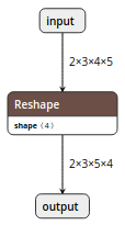
However, I got the following complicated model instead:

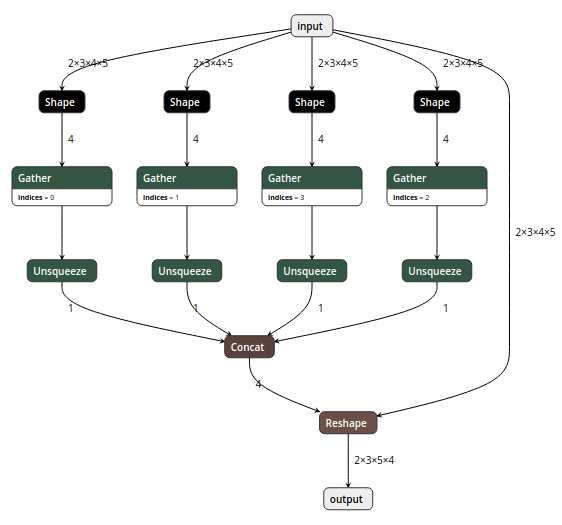
Our solution

ONNX Simplifier is presented to simplify the ONNX model. It infers the whole computation graph and then replaces the redundant operators with their constant outputs (a.k.a. constant folding).

Features

At its core onnxsim runs a fixed point of shape inference, graph optimization and constant folding until the model stops changing. Around that it offers:

• Constant folding. Evaluates the constant parts of the graph and replaces redundant operators with their computed outputs. By default initializers count as constants; pass --initializers-as-non-constants (Python: initializers_as_constants=False) to keep weights as tunable tensors so nodes rooted only at initializers — and value-baking fusions such as fuse BatchNorm into Conv — are left untouched.
• Graph optimization passes. Runs onnx-optimizer's fusions and eliminations (e.g. fuse BatchNorm into Conv). List them with onnxsim --list-default-optimizers; skip all or some with --skip-optimization [pass ...]. A pass not in the default set (typically a graph-shape rewrite rather than a pure node reduction, e.g. a defusion) can be requested explicitly with --enable-optimization pass [pass ...] (Python: extra_optimizers=); list those with --list-other-optimizers.
• Shape inference. Propagates tensor shapes through the graph — including partial shape evaluation via ONNX data propagation — to unlock more folding.
• Correctness checking. Optionally validates the simplified model against the original on N random inputs (the positional check_n argument, with configurable --check-rtol/--check-atol). Choose how the generated inputs are filled with --input-fill (Python: input_fill=): random (uniform [0, 1), the default), ones, zeros or arange.
• Fixed and dynamic input shapes. Pin a dynamic model's shapes for simplification/checking with --overwrite-input-shape and --test-input-shape.
• Custom operators. Keeps custom ops (TensorRT plugins, vendor domains, or custom ops in the default ONNX domain) unchanged and picks up schemas registered via onnx.defs.register_schema automatically.
• Opset conversion. Upgrade or downgrade the model's opset while simplifying with --target-opset.
• Function inlining. Flatten the model's local (model-defined) functions into the main graph before simplifying with --inline-functions (Python: inline_functions=True), so the optimizer, shape inference and constant folding can see through function calls. Schema-defined (built-in) functions are left alone.
• Custom rewriters. Plug your own rewriting logic into the fixed point with custom_rewriter, or express data-only FunctionProto rules that also run from the C and Rust bindings.
• Safetensors / GGUF archives. Export a model to a standalone .safetensors or .gguf file (graph + weights in one ecosystem-standard archive) and import it back, from every binding.
• Transformers export. Export a Hugging Face transformers model straight to a simplified ONNX deployment directory with onnxsim.export_transformers_model().
• Diffusion model export. Export a Hugging Face diffusers pipeline (Stable Diffusion, SDXL, ...) straight to a simplified ONNX deployment directory with onnxsim.export_diffusion_model().
• Detectron2 export. Trace a Detectron2 model (Faster/Mask/Keypoint R-CNN, RetinaNet, ...) to ONNX and simplify it with onnxsim.export_detectron_model().
• SAM 2 export. Trace a Meta SAM 2 image encoder and prompt/mask decoder to ONNX and simplify both with onnxsim.export_sam2_model().
• DriveTransformer export. Trace a DriveTransformer end-to-end autonomous-driving model to ONNX and simplify it with onnxsim.export_drivetransformer_model().
• Deploying to Axelera Metis devices. Safe to run ahead of Voyager SDK's own deploy.py: its Focus/space-to-depth and flattened-FC-head detectors, and any custom decode ops, survive simplify().
• Quantization-aware fine-tuning. Recover accuracy a quantization lost with onnxsim.apply_qat(): label-free, block-wise fine-tuning of the fp32 weights themselves against the float model's own activations, over any block topology --- and, with learn_activation_scales=True, of quantize_static's activation quantizers jointly with them. The training step is emitted as an ONNX graph, so it runs on a GPU, an NPU execution provider or WebGPU via step_providers=. The same loop with the fake-quantizer removed is onnxsim.apply_block_finetune() -- plain block-wise distillation of a model's own float weights against a reference model, for a model something else (a pruning, a requantization) already changed.
• Subgraph simplification. Simplify If/Loop/Scan subgraph bodies too with --include-subgraph.
• MLIR export. Hand the simplified model to torch-mlir (Torch dialect) or onnx-mlir (ONNX dialect) with --emit-mlir (Python: onnxsim.export_mlir) — a bridge into MLIR-based compiler stacks (torch-mlir, IREE, onnx-mlir). Both backends are optional.
• Core ML export. Convert the simplified model to a Core ML .mlpackage/.mlmodel with --emit-coreml (Python: onnxsim.export_coreml), via a built-in ONNX-to-MIL translator and coremltools' MIL-to-Core-ML backend. coremltools is optional.
• TensorFlow Lite export. Convert the simplified model to a .tflite flatbuffer with --emit-tflite (Python: onnxsim.export_tflite), via a built-in ONNX-to-TensorFlow translator and tf.lite.TFLiteConverter. TensorFlow is optional; pass --tflite-backend onnx2tf to route through onnx2tf instead for far broader op coverage.
• Large-model handling. Guard against blow-up from ops like Tile/ ConstantOfShape (--no-large-tensor), read and write external-data models, and eliminate unused outputs (--unused-output).
• Many ways to run it. A zero-install web version, a Python package and onnxsim CLI, a C API, and a Rust wrapper — all sharing the same C++ core. onnxruntime is optional; onnxsim falls back to the onnx reference evaluator when it isn't installed.

Getting started

Web version

We have published ONNX Simplifier on GitHub pages. It works out of the box and doesn't need any installation. Note that it runs in the browser locally and your model is completely safe.

Python version

pip3 install -U pip && pip3 install onnxsim

Then

onnxsim input_onnx_model output_onnx_model

For more advanced features, try the following command for help message

onnxsim -h

onnx is the only required dependency. Everything else is an extra, installed only if you want it -- among them rich, which is used purely to colour and box the terminal reports (the original-vs-simplified table, the memory plan, the graph diff, CLI warnings). Without it those print as plain-text ASCII tables and the simplified models are byte-for-byte the same:

pip3 install "onnxsim[rich]"

Pre-release builds from TestPyPI

Development builds from master are published to TestPyPI by the daily CI workflow when there are new commits, or on demand. To try the latest available pre-release, install the required dependency from PyPI first, then install onnxsim from TestPyPI:

python3 -m pip install --upgrade onnx
python3 -m pip install --upgrade --pre --no-deps --index-url https://test.pypi.org/simple/ onnxsim

--pre allows development versions and --upgrade updates an existing installation. --no-deps keeps dependency downloads on PyPI, since TestPyPI has a separate package collection. These builds contain unreleased changes; use the regular PyPI installation above for stable releases.

Node.js version

The same WebAssembly build backing the web version above is also published as an npm package, for JavaScript tooling that wants ONNX simplification without a native build step or a Python runtime. See npm/onnxsim/README.md for usage.

npm install onnxsim

Demonstration

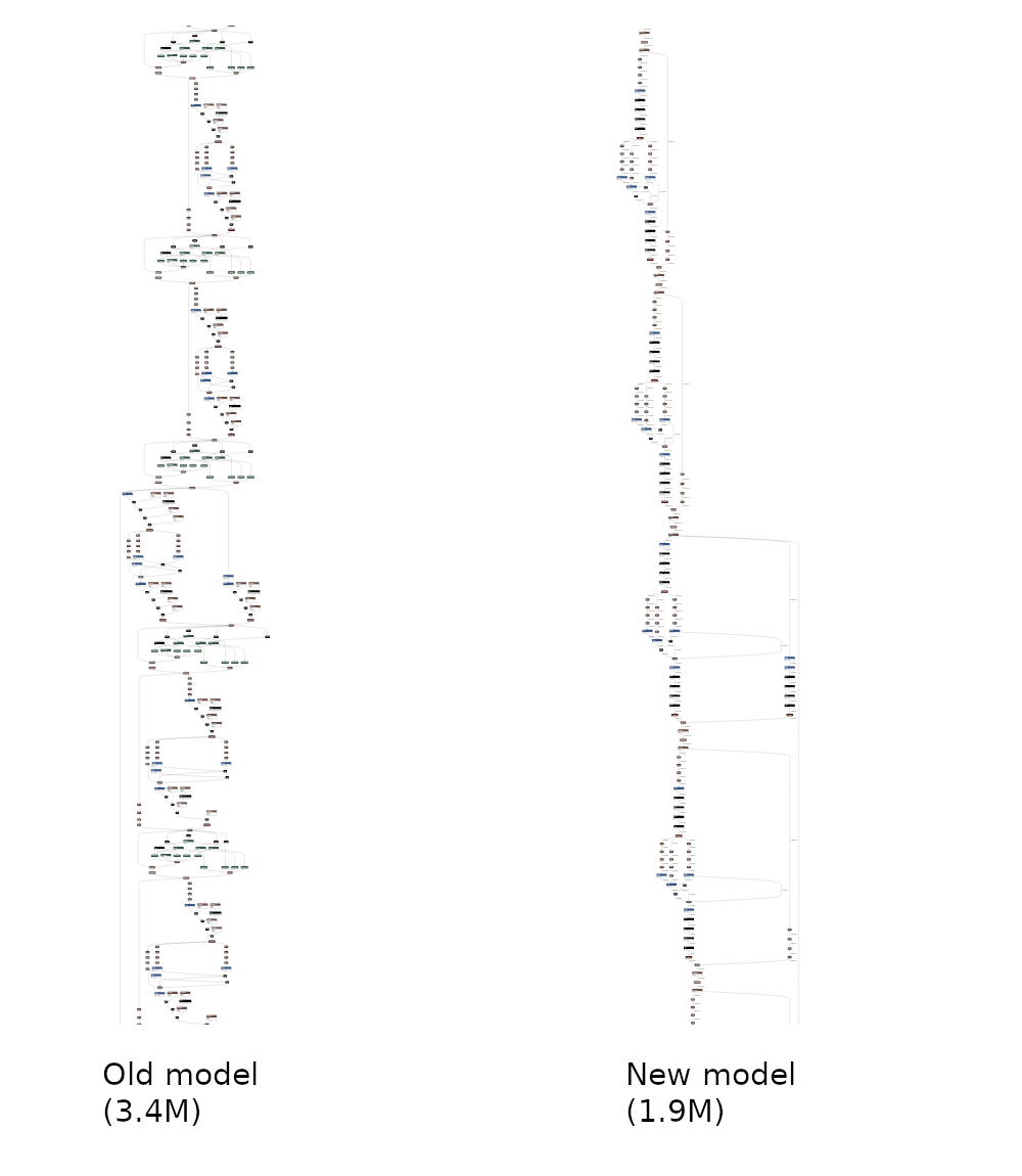
An overall comparison between a complicated model and its simplified version:

In-script workflow

If you would like to embed ONNX simplifier python package in another script, it is just that simple.

import onnx
from onnxsim import simplify

# load your predefined ONNX model
model = onnx.load(filename)

# convert model
model_simp, check = simplify(model)

assert check, "Simplified ONNX model could not be validated"

# use model_simp as a standard ONNX model object

You can see more details of the API in onnxsim/onnx_simplifier.py

Custom operators

Models that contain custom operators, such as TensorRT plugins (BatchedNMS_TRT, EfficientNMS_TRT, ...), are supported. onnxsim keeps these ops unchanged and simplifies the rest of the graph around them. This works whether the custom op lives in a vendor-specific domain (e.g. TRT) or in the default ONNX domain, so you no longer need to manually move it into a custom domain to get past validation (issues #107 and #220).

onnxsim also ships schemas out of the box for a few specific custom-op families, so shape inference propagates through them with no setup at all: ONNX Runtime's com.microsoft quantized/contrib ops, mmdeploy/mmcv/BEVDet's custom ops, and -- see docs/qonnx-brevitas-interop.md -- Brevitas's native QONNX export format (Quant/BipolarQuant/Trunc/FloatQuant, in the qonnx.custom_op.general or finn.custom_op.general domain). A Brevitas QAT export's learned quantizers are also picked up by onnxsim.qat_interop's ingest path (quantize_static_keeping_qdq_scales), the same as a QDQ-exported QAT model's -- see that doc and the "Quantization-aware fine-tuning" section below.

If you describe your custom operator to ONNX with onnx.defs.register_schema, onnxsim picks that schema up automatically: onnxsim links its own copy of ONNX, so its operator registry is separate from the onnx Python module's, and every simplify call imports the schemas you registered into onnxsim's registry before validating the model (issue #326). You can also trigger the import explicitly with onnxsim.import_onnx_schemas(), or turn the automatic import off with onnxsim.simplify(model, import_custom_schemas=False) (CLI: --skip-schema-import).

import onnx
import onnxsim

# Teach ONNX about your custom operator.
onnx.defs.register_schema(my_op_schema)

# simplify() imports the schema into onnxsim automatically.
model_simp, check_ok = onnxsim.simplify(model)

If a registered schema also has a type/shape-inference function (set via onnx.defs.OpSchema.set_type_and_shape_inference_function), onnxsim registers a trampoline that calls it back through onnx.shape_inference.infer_node_outputs during simplification, so the custom operator's output shapes are inferred too. Custom operators without an inference function are still imported; shape inference simply flows past them.

Changing the opset version

You can upgrade (or downgrade) the model's opset version while simplifying. Pass target_opset_version to simplify (CLI: --target-opset) and onnxsim converts the default ONNX domain to that opset — using onnx's own version converter — before running the simplification, so any redundant nodes the conversion introduces get cleaned up too.

import onnx
import onnxsim

model = onnx.load(filename)

# Convert the model to opset 18 and simplify it.
model_simp, check = onnxsim.simplify(model, target_opset_version=18)

On the command line:

onnxsim input_onnx_model output_onnx_model --target-opset 18

When target_opset_version is left unset (the default), the model's opset version is preserved.

The conversion runs inside onnxsim's C++ core, so every binding shares it — the Python package, the C API and its Rust wrapper (Options::target_opset_version), the standalone onnxsim binary (--target-opset), and the web version (the "target opset version" field).

Exporting to MLIR (torch-mlir / onnx-mlir)

Downstream compiler stacks built on MLIR — torch-mlir, IREE on top of it, and onnx-mlir — consume models as MLIR rather than as an ONNX ModelProto. onnxsim can bridge the gap: after simplifying, it emits the model as MLIR in one of two dialects, chosen with --mlir-target (Python: the target argument):

• torch (default) — Torch-dialect MLIR via torch-mlir's pure-Python ONNX importer.
• onnx — ONNX-dialect MLIR via the onnx-mlir compiler binary.

Simplifying first is the point — constant folding and the optimizer passes collapse the shape-manipulation subgraphs the importer would otherwise translate op by op, so the emitted MLIR is smaller and closer to what the compiler needs.

Both backends are optional (just like onnxruntime for constant folding): neither is imported/located unless you actually emit MLIR.

torch-mlir (Torch dialect)

Install torch-mlir:

pip install torch-mlir

Prebuilt wheels are listed at .

From the CLI, add --emit-mlir. Passed without a path it writes the MLIR next to the output model with a .mlir extension; pass a path to choose the location:

# writes simplified.onnx and simplified.mlir
onnxsim input.onnx simplified.onnx --emit-mlir

# choose the MLIR path explicitly
onnxsim input.onnx simplified.onnx --emit-mlir model.mlir

From Python, onnxsim.export_mlir converts a model (typically the output of simplify) and returns the MLIR text, optionally writing it to a file:

import onnx
import onnxsim

model = onnx.load("input.onnx")
model_simp, ok = onnxsim.simplify(model)
assert ok

# Return the MLIR as a string...
mlir_text = onnxsim.export_mlir(model_simp)
# ...and/or write it to a file.
onnxsim.export_mlir(model_simp, "model.mlir")

onnx-mlir (ONNX dialect)

onnx-mlir has no pip-installable importer, so this backend shells out to the onnx-mlir compiler binary (--EmitONNXIR). Build or install it from , then make it discoverable — put onnx-mlir on your PATH, set ONNX_MLIR_HOME to its install prefix (the binary is expected at $ONNX_MLIR_HOME/bin/onnx-mlir), set ONNX_MLIR to the binary path, or pass the path explicitly.

# locate onnx-mlir via PATH / ONNX_MLIR_HOME / ONNX_MLIR
onnxsim input.onnx simplified.onnx --emit-mlir --mlir-target onnx

# or point at the binary directly
onnxsim input.onnx simplified.onnx --emit-mlir model.mlir \
  --mlir-target onnx --onnx-mlir /path/to/onnx-mlir

mlir_text = onnxsim.export_mlir(model_simp, target="onnx")
# with an explicit binary path:
onnxsim.export_mlir(model_simp, "model.mlir", target="onnx",
                    onnx_mlir="/path/to/onnx-mlir")

export_mlir accepts a few keyword arguments, forwarded to the selected backend — e.g. opset_version to run ONNX's version converter first (both targets prefer recent opsets), verify=False (torch) to skip MLIR verification, and emit / extra_args (onnx) to change the onnx-mlir emit flag or pass extra compiler options. See onnxsim/mlir_export.py for the full signatures.

Exporting to Core ML

Apple platforms want the graph as a Core ML model instead of ONNX or MLIR. coremltools dropped its own ONNX frontend in version 7 (it only converts TensorFlow/PyTorch models, or an in-memory MIL program) — there's no off-the-shelf "convert this ONNX model" call left to lean on, so onnxsim ships its own ONNX-to-MIL translator and hands the result to coremltools' MIL-to-Core-ML backend to produce the actual model. It covers a practical subset of ONNX ops (conv/pooling/normalization, matmul/gemm, elementwise math, reshapes, reductions, GridSample, and more — see coreml_export.SUPPORTED_ONNX_OPS); a node whose op isn't supported raises a clear error naming the op, rather than silently producing a wrong model. Feeding in a simplified model is the point, same as with MLIR export: onnxsim's constant folding turns more of the graph into plain initializers, so more of it lands on the translator's supported-op list.

coremltools is optional, just like onnxruntime for constant folding: it isn't imported unless you actually export to Core ML.

pip install coremltools

Converting an ONNX model to MIL / Core ML needs no macOS-specific functionality (MIL construction and .mlpackage serialization are pure Python/protobuf), so it runs the same on Linux, macOS, or Windows. Only loading the produced model back for a prediction needs Core ML's runtime, i.e. an Apple OS — pass skip_model_load=False (Python) once you're on macOS to get a model that's ready to call .predict() on; the default (skip_model_load=True) lets conversion succeed everywhere else too.

Graph inputs must have fully static shapes (dynamic axes aren't supported).

From the CLI, add --emit-coreml. Passed without a path it writes the model next to the output model with a .mlpackage/.mlmodel extension; pass a path to choose the location:

# writes simplified.onnx and simplified.mlpackage
onnxsim input.onnx simplified.onnx --emit-coreml

# choose the path and the legacy .mlmodel format explicitly
onnxsim input.onnx simplified.onnx --emit-coreml model.mlmodel --coreml-format neuralnetwork

From Python, onnxsim.export_coreml converts a model (typically the output of simplify) and returns the coremltools.models.MLModel, optionally saving it:

import onnx
import onnxsim

model = onnx.load("input.onnx")
model_simp, ok = onnxsim.simplify(model)
assert ok

# Return the MLModel...
mlmodel = onnxsim.export_coreml(model_simp)
# ...and/or save it to a .mlpackage (or .mlmodel with convert_to="neuralnetwork").
onnxsim.export_coreml(model_simp, "model.mlpackage")

export_coreml accepts a few keyword arguments: convert_to ("mlprogram", the default, or the legacy "neuralnetwork"), compute_units (which devices the model may run on, e.g. "CPU_ONLY"), compute_precision, minimum_deployment_target (e.g. "iOS16"), io_dtype (see below), and skip_model_load (see above). See onnxsim/coreml_export.py for the full signature.

io_dtype="fp16" (CLI: --coreml-io-dtype fp16) declares the model's float inputs and outputs float16 instead of float32. An ML Program already computes in float16, so the float32 default only buys a conversion in each direction on every call, over twice the bytes — with no accuracy difference, since a float32 output is just an upcast of the float16 value Core ML computed either way. It's worth most where the same large float tensors cross the boundary repeatedly, as a transformer decoder's KV cache does on every generated token. Requires convert_to="mlprogram" and raises the deployment target to iOS16/macOS13 when one isn't given. See scripts/apple/README.md's "fp16 model interface" section.

Exporting to TensorFlow Lite

Mobile/embedded runtimes built on TensorFlow want the graph as a .tflite flatbuffer instead of ONNX or Core ML. onnx-tensorflow/onnx-tf (the project that used to fill this gap) has been unmaintained for years and only tracks very old opsets, so -- same situation as Core ML after coremltools dropped its own ONNX frontend -- onnxsim ships its own ONNX-to-TensorFlow translator: it builds the equivalent computation with plain TensorFlow ops inside a tf.function, traces it into a concrete function, and hands that to tf.lite.TFLiteConverter to produce the actual .tflite model. It covers a practical subset of ops (conv/pooling/normalization incl. LayerNormalization, matmul/gemm, elementwise math incl. comparisons, reshapes, reductions, TopK, Resize, ConvTranspose, ScatterND and GridSample -- see tflite_export.SUPPORTED_ONNX_OPS); a node whose op isn't supported raises a clear error naming the op, rather than silently producing a wrong model. Feeding in a simplified model is the point, same as with the other export backends: onnxsim's constant folding turns more of the graph's shape-manipulation subgraphs into plain initializers, which this translator needs at conversion time for things like a Reshape's target shape or a Slice's bounds.

TensorFlow is optional, just like onnxruntime for constant folding and coremltools for Core ML export: it isn't imported unless you actually export to TFLite.

pip install tensorflow

TensorFlow Lite's own op kernels are NHWC-only, while ONNX's conv/pool ops are NCHW; this translator keeps the graph's public tensors in ONNX's NCHW layout and transposes to/from NHWC only around the ops that need it, so no manual layout conversion is required on your part. Graph inputs must have fully static shapes (dynamic axes aren't supported) -- pin them first with --overwrite-input-shape/--test-input-shape if needed.

From the CLI, add --emit-tflite. Passed without a path it writes the model next to the output model with a .tflite extension; pass a path to choose the location:

# writes simplified.onnx and simplified.tflite
onnxsim input.onnx simplified.onnx --emit-tflite

# choose the path explicitly, and enable TFLite's default post-training
# (dynamic-range) quantization
onnxsim input.onnx simplified.onnx --emit-tflite model.tflite --tflite-optimize

From Python, onnxsim.export_tflite converts a model (typically the output of simplify) and returns the serialized .tflite flatbuffer (bytes), optionally writing it to a file:

import onnx
import onnxsim

model = onnx.load("input.onnx")
model_simp, ok = onnxsim.simplify(model)
assert ok

# Return the flatbuffer bytes...
tflite_model = onnxsim.export_tflite(model_simp)
# ...and/or write it to a file.
onnxsim.export_tflite(model_simp, "model.tflite")

export_tflite accepts an optimizations keyword argument, forwarded to tf.lite.TFLiteConverter.optimizations (e.g. ["DEFAULT"], what --tflite-optimize sets, to enable post-training dynamic-range quantization). See onnxsim/tflite_export.py for the full signature.

A few ops have a correct translation but no TFLite kernel of their own (Atan is one) and fail conversion loudly at the converter. For a model whose only unmappable op is such a CPU-side tail (e.g. BEVFormer box-yaw decoding), pass flex_ops=True (CLI: --tflite-flex) to partition those kernels to TensorFlow Flex on the CPU while everything else stays a TFLite builtin. A Flex model cannot target the Edge TPU (flex_ops is mutually exclusive with --tflite-int8).

Einsum is decomposed before any of this

None of the hand-written translators (Core ML, TFLite, WebNN) has an Einsum kernel, and a surprising share of real graphs are made of it: PyTorch emits it for linear layers, attention projections, and ray/sample contractions, which is most of a NeRF, MLP or attention graph. Rather than teach each translator the op, onnxsim rewrites the batched-matrix-multiply form once, at the ONNX level, on the way into every one of them (onnxsim/einsum_decompose.py):

Einsum(bnc,cd->bnd)  ->  MatMul        # already in matmul order, no transpose
Einsum(bij,bjk->bik) ->  MatMul        # shared batch axis leads both operands
Einsum(mj,nj->mn)    ->  Transpose, MatMul

The rewrite is exact: ONNX MatMul computes A[batch, m, k] @ B[batch, k, n], which is by construction the einsum's own output order, so no output-side reshape or transpose is ever needed and an operand already in matmul order contributes no Transpose.

Deliberately not rewritten: a diagonal, a trace, an outer product, a reduction to a scalar, or a batch axis only one operand carries. Those are left exactly as they were, so the exporter still raises its usual "unsupported op" error naming the op -- never a silently wrong model. backend="onnx2tf" and the MLIR path, which delegate, cover those without this caveat.

The function is importable on its own if you want the rewrite without exporting:

from onnxsim.einsum_decompose import decompose_einsum

model = decompose_einsum(model)

A broader-coverage backend: onnx2tf

The built-in translator above covers a practical op subset. For a model that hits an unsupported op, pass backend="onnx2tf" (CLI: --tflite-backend onnx2tf) to route the conversion through onnx2tf instead -- a separate, actively maintained project with far broader op coverage (~200 ops) and years of production hardening across real-world model zoos.

pip install onnx2tf

onnx2tf is a much heavier dependency than the builtin backend needs (it pulls its own TensorFlow, onnxruntime, onnx-graphsurgeon, and a couple dozen small *4onnx helper packages), and it changes the model's public input/output tensor layout to channel-last by default -- it converts every tensor of rank >= 3 to that convention, not just 4-D image tensors, unlike the builtin backend which always keeps ONNX's own declared shapes. Pass onnx2tf's own keep_ncw_or_nchw_or_ncdhw_input_names (a list of input names to keep in their original ONNX layout) as an extra keyword argument if you need specific inputs to keep their original layout.

onnxsim input.onnx simplified.onnx --emit-tflite --tflite-backend onnx2tf

tflite_model = onnxsim.export_tflite(model_simp, backend="onnx2tf")

--tflite-optimize/optimizations only applies to the builtin backend; use onnx2tf's own quantization options (forwarded as extra keyword arguments, e.g. output_integer_quantized_tflite=True) instead. See onnxsim/onnx2tf_export.py for the full signature and onnx2tf's own documentation for its option list.

Running on the Coral Edge TPU

The Edge TPU only runs fully 8-bit quantized models compiled with edgetpu_compiler. onnxsim covers that tail of the pipeline (see onnxsim/edgetpu_export.py):

# 1. full-integer quantization with quantized I/O (TensorFlow required)
onnxsim input.onnx simplified.onnx --emit-tflite model.tflite \
  --tflite-int8 --tflite-io-dtype uint8

# 2. compile for the Edge TPU (needs the edgetpu_compiler binary)
onnxsim input.onnx simplified.onnx --emit-tflite model.tflite --tflite-edgetpu

--tflite-edgetpu implies --tflite-int8 and writes model_edgetpu.tflite next to the .tflite file (pass a path to choose it), printing per-operator TPU/CPU statuses from the compiler log. Calibration uses uniform-random data (--tflite-calibration-samples N, default 100) unless you pass real representative inputs via the Python API's representative_dataset=. --tflite-edgetpu-check statically checks the simplified model against the Edge TPU requirements (static shapes, supported ops) before converting.

Channel order: --tflite-layout nhwc for larger models

By default the builtin translator keeps public tensors in ONNX's NCHW order and transposes around each conv/pool. That is free for small models (TF folds the interior transposes, leaving just the boundary pair), but the Edge TPU compiler refuses the NCHW entry transpose above modest activation sizes (measured: a 64-channel 32x32 conv fails with large activation tensors, while the identical channel-last graph maps fully; the exit transpose is harmless). --tflite-edgetpu-check warns when a model enters that envelope (4-D activations with 8+ channels and 65536+ elements, inputs and inferred intermediates).

Pass --tflite-layout nhwc (Python: io_layout="nhwc") to carry 4-D tensors channel-last end to end instead: public 4-D I/O changes dimension order to NHWC, but conv/pool/concat emit no transposes at all (verified: the 64ch 32x32 model compiles with every op mapped). Feed NHWC-ordered inputs at inference and when supplying representative_dataset=.

Peak performance on the device itself is characterized in scripts/edgetpu/README.md: a 6-model benchmark suite (pointwise/dense/depthwise/FC workloads) with exact MACs, edgetpu_compiler mapping + on-chip memory stats, and a roofline over USB link speeds — plus a ready-to-run on-device timing script. Short version: the 4 TOPS spec peak is unattainable sustained; expect ~1.6 TOPS for ideal dense compute-bound models on USB3, 0.1–0.4 TOPS for realistic mobile CNNs, and link-bound numbers on USB 2.0.

model_simp, ok = onnxsim.simplify(model)
assert ok

# Check first (onnx only, no other dependency)...
report = onnxsim.check_onnx_for_edgetpu(model_simp)
print(report.summary())

# ...then quantize, compile, and run via LiteRT.
edgetpu = onnxsim.export_edgetpu(model_simp, "model_edgetpu.tflite")
print(edgetpu.compile_result.summary())

out = onnxsim.run_litert("model_edgetpu.tflite", {"x": x_uint8}, use_edgetpu=True)

Inference runs on LiteRT (pip install ai-edge-litert, the successor to tflite-runtime); use_edgetpu=True loads the libedgetpu delegate for on-device execution (see onnxsim.edgetpu_setup_hint() for the runtime/udev setup). Without a device, the same call with use_edgetpu=False runs the quantized model on CPU.

Constant folding on the GPU (CUDA execution provider)

onnxsim constant-folds by running the foldable sub-graphs through ONNX Runtime. By default it uses the CPU execution provider, which is always available and gives deterministic results. For large models it can be much faster to fold on an NVIDIA GPU. Pass providers to simplify to choose the ONNX Runtime execution providers, in priority order:

import onnx
import onnxsim

model = onnx.load(filename)

# Fold on the GPU, falling back to CPU for ops CUDA cannot run.
model_simp, check = onnxsim.simplify(
    model, providers=["CUDAExecutionProvider", "CPUExecutionProvider"]
)

On the command line:

# Explicit provider list (priority order):
onnxsim input_onnx_model output_onnx_model \
    --providers CUDAExecutionProvider CPUExecutionProvider

# Or the shortcut, equivalent to the line above:
onnxsim input_onnx_model output_onnx_model --cuda

Keeping CPUExecutionProvider last is recommended: ONNX Runtime falls back to it for any operator the GPU provider cannot run. Each provider entry may also be a (name, options) tuple, exactly as onnxruntime.InferenceSession accepts it, for example to pin a specific device_id:

model_simp, check = onnxsim.simplify(
    model,
    providers=[("CUDAExecutionProvider", {"device_id": 1}), "CPUExecutionProvider"],
)

The CUDA execution provider requires the GPU build of ONNX Runtime (pip install onnxruntime-gpu). On AMD ROCm hardware the same providers mechanism reaches ROCMExecutionProvider (pip install onnxruntime-rocm) and MIGraphXExecutionProvider (pip install onnxruntime-migraphx, or the onnxruntime-ep-migraphx plugin on newer ROCm stacks -- see scripts/amd/README.md), for constant folding and -- via step_providers= -- for the QAT/block-finetune/training step graphs as well:

model_simp, check = onnxsim.simplify(
    model, providers=["MIGraphXExecutionProvider", "CPUExecutionProvider"]
)

If you request a provider the installed ONNX Runtime does not offer, onnxsim raises a ValueError listing the available providers instead of silently folding on the CPU. When providers is left unset (the default), folding runs on the CPU.

examples/cuda_feature_tests/ has a notebook exercising this end to end (folding, the CLI, device_id pinning, DLPack CUDA tensors, provider validation) against a real GPU -- open it in Colab and run it by hand whenever you want to check these on an actual NVIDIA GPU; it is not wired into CI.

Constant folding with the AMD NPU (Vitis AI execution provider)

The same providers mechanism works for AMD's Ryzen AI NPU: its ONNX Runtime provider is called VitisAIExecutionProvider, and it partitions the graph into NPU/CPU subgraphs transparently (unsupported ops fall back to the CPU, so keep CPUExecutionProvider last exactly as with CUDA):

model_simp, check = onnxsim.simplify(
    model,
    providers=[
        ("VitisAIExecutionProvider", {"config_file": "vaip_config.json"}),
        "CPUExecutionProvider",
    ],
)

Two differences from CUDA matter. First, the provider never comes from PyPI: the stock onnxruntime / onnxruntime-gpu wheels do not ship it. It comes from AMD's Ryzen AI Software bundle (XRT NPU drivers plus the ryzen_ai venv, which contains the Vitis AI EP build of ONNX Runtime) -- see AMD's Linux install guide and the Vitis AI EP docs. Without that bundle VitisAIExecutionProvider is absent from ort.get_available_providers() and onnxsim raises a ValueError pointing at the Ryzen AI installer (rather than at onnxruntime-gpu). Second, the provider options (config_file for BF16 models, target/xclbin for INT8, cache_dir/cache_key to reuse a compiled model) need the (name, options) tuple form above, which only the Python API offers -- the CLI's --providers takes bare provider names. NPU compilation happens at session creation and can take minutes the first time; the cache options avoid repaying it.

In practice, prefer to keep constant folding itself on the CPU (fold groups are tiny shape/index subgraphs where NPU compile time dwarfs any speedup, and CPU folding is deterministic) and use the NPU for running the full model -- correctness checking (check_n), backend.run_model / backend.Runner, or the QAT/training loops' step_providers=.

Quantized models on the NPU

The EP executes INT8 (and, via config_file, BF16-compiled) graphs; which subgraphs land on the NPU is decided by its own fusion passes. The recommended INT8 recipe is AMD Quark's XINT8 config (pip install amd-quark, no AMD login needed), then onnxsim's Vitis AI legalizer, then the EP with target=X2 (the backend for Strix/KrackanPoint; no xclbin):

from quark.onnx import ModelQuantizer, QConfig

# 1. Quantize (Quark XINT8: UINT8 activations / INT8 weights, power-of-2 scales).
quantizer = ModelQuantizer(QConfig.get_default_config("XINT8"))
quantizer.quantize_model("fp32.onnx", "int8.onnx", calib_reader)

# 2. Legalize for the NPU (fixes what the EP can't take -- see below).
import onnxsim
model = onnxsim.legalize_for_vitisai(onnx.load("int8.onnx"))
print(onnxsim.check_vitisai_support(model))  # [] means NPU-safe

# 3. Run on the NPU (inside the ryzen_ai venv, XRT set up).
import onnxruntime as ort
sess = ort.InferenceSession(
    model.SerializeToString(),
    providers=[("VitisAIExecutionProvider", {"target": "X2"}),
               "CPUExecutionProvider"],
)

Two sharp edges, both measured on Strix Halo / Ryzen AI 1.8:

• Conv without explicit attributes aborts the process. A Conv relying on ONNX defaults (no strides/pads/dilations/kernel_shape/ group -- exactly what stock onnxruntime quantization and Quark emit) dies in XIR conversion (conv2d: Attr stride REQUIRED) instead of falling back. legalize_for_vitisai materializes them (resolving the weight through DequantizeLinear chains), turning the abort into an NPU offload -- verified bit-exact vs CPU on a quantized conv probe, and on Quark XINT8/A8W8 outputs alike.
• The EP rejects bf16-typed graphs (INVALID_GRAPH); BF16 execution means an fp32 graph plus config_file, never a bf16 graph. LSTM nodes segfault session creation -- keep those on CPU. Standalone activations/norms/softmax and data-movement ops simply fall back to CPU by design; only conv/pool/matmul-centred subgraphs offload (check_vitisai_support flags exactly the hard-failure cases above).

Profiling the optimization

Simplification alternates a handful of transforms -- shape inference, the onnx-optimizer passes, constant folding and any custom rewriter -- to a joint fixed point. To see where the time and memory go, pass profile to simplify (or --profile on the command line). onnxsim then measures each fixed-point function's wall-clock and CPU duration and the peak resident memory reached while it runs, prints a per-function summary, and writes a Chrome Trace Event Format JSON. Open that file in chrome://tracing or at ui.perfetto.dev to view it as a flame graph: the nested fixed points appear as parent spans and the individual transforms as their children, one box per invocation, annotated with peak RSS and CPU time.

Constant folding's actual work is running the model through ONNX Runtime, so those session runs are profiled too. Each fold group appears under FoldConstant as an OrtSession span, which times running that group's sub-model through the inference executor. This works for every binding, since it wraps the one call site common to both the built-in ONNX Runtime executor and the Python executor that simplify() uses. When the built-in executor runs, the OrtSession span is split further into OrtSessionInit (building the session, where ONNX Runtime loads the graph and usually the dominant cost) and OrtSessionRun (the inference). This makes it easy to see how much of simplification time is spent inside ONNX Runtime versus in shape inference and the optimizer passes.

import onnx
import onnxsim

model = onnx.load(filename)

# Write the trace to profile.json (open it in chrome://tracing or ui.perfetto.dev).
model_simp, check = onnxsim.simplify(model, profile="profile.json")

On the command line:

# Give a path, or omit it to use onnxsim_profile.json in the current directory.
onnxsim input_onnx_model output_onnx_model --profile profile.json

The printed summary looks like:

onnxsim profiling summary (per fixed-point function)
-------------------------------------------------------------------------------------
function                calls     wall(ms)      cpu(ms) max wall(ms)    peak(MiB)
-------------------------------------------------------------------------------------
Simplify                    1       260.59       270.93       260.59       112.95
  Pipeline                  3       259.75       269.67       100.76       112.94
    OptAndShape             3       158.63       165.13        53.20       101.43
    FoldConstant            3       100.36       103.78        47.69       112.93
      Optimize              3       112.56       116.99        37.77       101.42
      InferShapes           3        45.46        47.10        15.22        78.68
      OrtSession           12        71.44        74.02        18.31       112.93
        OrtSessionInit     12        58.02        60.11        15.90       112.93
        OrtSessionRun      12         9.85        10.42         2.71       109.10
-------------------------------------------------------------------------------------

(OrtSessionInit/OrtSessionRun show only when the built-in ONNX Runtime executor runs the fold; the Python simplify() path shows just OrtSession.)

calls is how many times a function ran across all fixed-point rounds, cpu(ms) is process CPU time (it can exceed wall time when constant folding runs multiple ONNX Runtime threads), and peak(MiB) is the highest process RSS observed while that function was on the stack (sampled by a lightweight background thread; tune the interval with ONNXSIM_PROFILE_INTERVAL_MS, default 5ms).

Profiling is implemented in onnxsim's C++ core and is driven by the ONNXSIM_PROFILE environment variable (the Python profile argument and the --profile flag just set it), so it also works from the C ABI and the Rust wrapper without any code change:

ONNXSIM_PROFILE=profile.json onnxsim input_onnx_model output_onnx_model

ONNX Runtime's own session profiler

The OrtSession span above times each folding session as a whole. For a finer, per-operator breakdown inside those sessions, turn on ONNX Runtime's own session profiler with ort_profile (or --ort-profile). This flips on SessionOptions.enable_profiling for the ONNX Runtime sessions onnxsim runs while simplifying (the constant-folding sessions, plus the correctness-check runs when check_n > 0), so each one writes ONNX Runtime's detailed per-kernel Chrome trace:

# Write onnxruntime session traces with the given file prefix.
model_simp, check = onnxsim.simplify(model, ort_profile="ort_profile")

onnxsim input_onnx_model output_onnx_model --ort-profile ort_profile

The value is a file prefix: ONNX Runtime writes one _.json per session, so a run that folds in several batches produces several files (open each in chrome://tracing or ui.perfetto.dev). It is independent of profile -- use either, or both together (profile for onnxsim's pipeline, ort_profile for what ONNX Runtime does inside each fold). Like profile, it is driven by an environment variable (ONNXSIM_ORT_PROFILE), so it works from every binding:

ONNXSIM_ORT_PROFILE=ort_profile onnxsim input_onnx_model output_onnx_model

Merging it into onnxsim's trace

Rather than juggling separate files, merge_ort_profile (or --merge-ort-profile) splices ONNX Runtime's per-operator events straight into onnxsim's profile trace, so each OrtSession span gets ONNX Runtime's operator-level detail lined up beneath it on its own onnxruntime track -- one unified flame graph. It implies profile (defaulting to onnxsim_profile.json), and ONNX Runtime's intermediate traces are captured to a temporary directory and removed after merging, so nothing is left behind. This works for every executor, including the Python one simplify() uses:

model_simp, check = onnxsim.simplify(model, profile="profile.json", merge_ort_profile=True)

onnxsim input_onnx_model output_onnx_model --profile profile.json --merge-ort-profile

The merge is also available from the C ABI, Rust and WASM bindings (which fold through the built-in ONNX Runtime executor): set the ONNXSIM_MERGE_ORT_PROFILE environment variable and it is done entirely in onnxsim's C++ core -- no Python needed. It implies ONNXSIM_PROFILE (defaulting to onnxsim_profile.json):

ONNXSIM_MERGE_ORT_PROFILE=1 onnxsim input_onnx_model output_onnx_model

Node-reduction plot

A profile trace also records how many nodes the graph holds right after every round of each fixed-point loop (Optimize, FoldConstant, and Rewrite when a custom_rewriter is given), as NodeCount counter events. onnxsim.profile_plot.plot_node_reduction (or --node-reduction-plot on the command line) turns those into a PNG with one subplot per loop -- node count against round index -- so you can see at a glance how many rounds each loop took and whether it converged (a flat tail) or hit the round cap (ONNXSIM_FIXED_POINT_ITERS, default 50) still descending. It needs matplotlib (pip install onnxsim[plot]):

model_simp, check = onnxsim.simplify(model, profile="profile.json")

from onnxsim.profile_plot import plot_node_reduction
plot_node_reduction("profile.json")  # -> profile.json_node_reduction.png

# Implies --profile if not given explicitly.
onnxsim input_onnx_model output_onnx_model --node-reduction-plot

Custom rewriters

Beyond the built-in optimizer passes, you can plug your own graph rewriting logic into simplification with the custom_rewriter parameter of simplify(). It accepts a callable

Callable[[onnx.ModelProto], Optional[onnx.ModelProto]]

that either returns a rewritten model or mutates the model in place and returns None. The callable runs inside onnxsim's simplification fixed point, interleaved with shape inference, the built-in optimizer and constant folding — so a rewrite can expose new optimization/folding opportunities and vice versa, and the whole pipeline iterates until it converges. onnxsim itself takes no dependency on any particular rewriting library; you bring your own.

Using onnx-rewriter (onnxscript.rewriter)

onnx-rewriter lets you express a subgraph pattern and its replacement as plain Python and have it matched and rewritten anywhere in the model. Install it alongside onnxsim:

pip3 install onnxscript

Then define a rule set and hand it to simplify via custom_rewriter. This example fuses MatMul + Add into a single Gemm:

import onnx
import onnxsim
from onnxscript.rewriter import pattern, rewrite

# The subgraph to match: y = MatMul(x, w) + b
def matmul_add_pattern(op, x, w, b):
    return op.Add(op.MatMul(x, w), b)

# What to replace it with: y = Gemm(x, w, b)
def gemm_replacement(op, x, w, b):
    return op.Gemm(x, w, b)

rules = pattern.RewriteRuleSet(
    [pattern.RewriteRule(matmul_add_pattern, gemm_replacement)]
)

model = onnx.load("model.onnx")
model_simp, check = onnxsim.simplify(
    model,
    custom_rewriter=lambda m: rewrite(m, pattern_rewrite_rules=rules),
)
assert check, "Simplified ONNX model could not be validated"

Because the rewriter runs every round of the fixed point, the fused Gemm above (and anything it unlocks) is folded and re-optimized together with the rest of the graph.

Skipping the copy when nothing is rewritten

The rewriter runs on every fixed-point round, including the final one where it has nothing left to do — and the fixed point always ends with at least one such no-op round to detect convergence. onnxsim hands the model to your callable as protobuf bytes and parses whatever comes back into a fresh ModelProto, so a rewriter that reports a rewritten model each round pays for that copy even when it changed nothing.

Return False to tell onnxsim that this round rewrote nothing; onnxsim then keeps the model it already has and skips the round-trip. Run the rules through onnx-ir's PassManager — onnxscript.rewriter.RewritePass wraps a rule set as an IR pass — and read the modified flag of the PassResult it returns. That flag is the reliable signal: an IR round-trip can reorder the serialized bytes even when no rule fires, so a byte comparison would falsely report a change.

from onnxscript import ir
from onnxscript.rewriter import RewritePass, pattern

rules = pattern.RewriteRuleSet(
    [pattern.RewriteRule(matmul_add_pattern, gemm_replacement)]
)
rewrite_pass = ir.passes.PassManager([RewritePass(rules)])

def apply_rules(model: onnx.ModelProto):
    model_ir = ir.serde.deserialize_model(model)
    result = rewrite_pass(model_ir)  # ir.passes.PassResult
    if not result.modified:
        return False  # no rule fired this round: skip the copy
    return ir.serde.serialize_model(result.model)

model_simp, check = onnxsim.simplify(model, custom_rewriter=apply_rules)

The plain lambda m: rewrite(m, pattern_rewrite_rules=rules) form still works — it just always returns a model, so onnxsim copies it back every round.

A few things to keep in mind:

• Keep the model schema-valid. After each rewrite onnxsim validates the model, so any op you introduce must be registered at the model's opset (for example Gelu only exists from opset 20). Custom-domain ops are fine — see Custom operators for registering their schemas.
• Match the opset your rules target. Convert the model to the opset your patterns expect (e.g. with onnx.version_converter) before simplifying if needed.
• You are not limited to onnx-rewriter. Any callable works — a hand-written pass over model.graph, an onnx-graphsurgeon edit, etc. — as long as it takes and returns a ModelProto.

From the C API and Rust

The custom rewriter lives in onnxsim's C++ core, so the C API and its Rust wrapper expose it too — the model is exchanged as serialized ModelProto bytes across the boundary instead of as an onnx.ModelProto object. In Rust, use simplify_with_rewriter (or simplify_path_with_rewriter) and pass a closure FnMut(&[u8]) -> Result>, E>: return Ok(None) when a round rewrote nothing (onnxsim skips the copy, matching the Python False sentinel), Ok(Some(bytes)) for the rewritten model, or Err(..) to abort.

let simplified = onnxsim::simplify_with_rewriter(
    &model_bytes,
    &onnxsim::Options::new(),
    |bytes: &[u8]| {
        // Decode `bytes`, rewrite, and return the new bytes — or Ok(None).
        let _ = bytes;
        Ok::<_, onnxsim::Error>(None)
    },
)?;

In C, pass an OnnxsimRewriteFn callback (and an optional matching free callback) to onnxsim_simplify / onnxsim_simplify_path; see onnxsim/capi/onnxsim_c_api.h for the contract. The only binding without it is the standalone CLI, which has no way to carry a user callback.

FunctionProto rules (works in every binding)

custom_rewriter takes a Python callable, so it only works from the Python binding. If instead you express a rule as pure data — a (pattern, replacement) pair of onnx.FunctionProto — onnxsim matches and applies it in its C++ core, so the same rule set also works from the C and Rust bindings with no dependency on onnxscript. The pattern's inputs are wildcards that bind to graph values, its body is the subgraph to match, and its outputs are rewired to the replacement's outputs. Build the FunctionProtos with onnx.parser.parse_function:

import onnx
import onnxsim
from onnx import parser

pattern = parser.parse_function("""

matmul_add_pattern (x, w, b) => (y)
{
    t = MatMul(x, w)
    y = Add(t, b)
}
""")
replacement = parser.parse_function("""

gemm_replacement (x, w, b) => (y)
{
    y = Gemm(x, w, b)
}
""")

model = onnx.load("model.onnx")
model_simp, check = onnxsim.simplify(
    model, function_rewrite_rules=[(pattern, replacement)]
)

This is enough to stand in for a hand-written onnxoptimizer pass: the rule above reproduces the built-in fuse_matmul_add_bias_into_gemm fusion. Skip the built-in pass and let the rule do it:

model_simp, check = onnxsim.simplify(
    model,
    skipped_optimizers=["fuse_matmul_add_bias_into_gemm"],
    function_rewrite_rules=[(pattern, replacement)],
)

A node attribute written @name (an ONNX-text ref attribute) is an attribute wildcard: it binds the matched node's attribute and is substituted into the replacement. function_rewrite_rules is mutually exclusive with custom_rewriter.

Many of onnxscript's ready-made common rewrite rules (e.g. matmul_add_to_gemm_rule, reshape_reshape_rule) are simple structural pattern→replacement rules that translate directly into a FunctionProto pair like the one above; see tests/test_function_rewriter_common_rules.py for worked examples that check parity against the onnxscript rule itself.

Instead of writing the ONNX text by hand you can author each side as an onnxscript.script function and call .to_function_proto() — a Python-typed attribute parameter (alpha: float) even compiles to the @name wildcard form:

from onnxscript import script
from onnxscript import opset18 as op

@script()
def matmul_add(a, b, c):
    return op.Add(op.MatMul(a, b), c)

@script()
def gemm(a, b, c):
    return op.Gemm(a, b, c)

model_simp, check = onnxsim.simplify(
    model,
    function_rewrite_rules=[(matmul_add.to_function_proto(), gemm.to_function_proto())],
)

See tests/test_function_rewriter_onnxscript_script.py for the @script approach, including the attribute-wildcard case. To reuse an existing onnxscript rule, its structural pattern method can be compiled to a FunctionProto through the same @script converter — tests/test_function_rewriter_compile_rule.py shows a small helper that does this (paired with a simple replacement), noting the boundary where a rewrite that derives attributes from the match can't be compiled that way.

From C, call onnxsim_simplify_with_rules with the serialized FunctionProto pairs (see onnxsim/capi/onnxsim_c_api.h); from Rust, use Options::function_rewrite_rule(pattern_bytes, replacement_bytes).

Capabilities and limits of the built-in matcher. It matches arbitrary connected DAG patterns with one or more outputs, tries both operand orders for the commutative binary ops (Add, Mul, …), matches attributes exactly or as @name wildcards, matches a pattern Constant against a byte-equal initializer, and refuses a rewrite that would break a value consumed outside the match. It does not (in this version) traverse If/Loop/Scan subgraph bodies, handle variadic/optional-input arity mismatches, match >2-operand commutative permutations, or evaluate attribute predicates — for those, the Python-only onnxscript.rewriter via custom_rewriter remains the richer option.

Safetensors / GGUF archives

Reading onnx-safetensors-styled models needs no special handling. onnx_safetensors.save_file/save_model/ load_file_as_external_data write an ordinary .onnx graph whose initializers use standard ONNX external data (location/offset/length) pointing into a real .safetensors file — the safetensors JSON header is simply skipped over by offset. That's exactly the external-data mechanism simplify() already reads (from a path or from onnx.load()), so a model produced by onnx-safetensors — or any other tool following the same convention — loads and simplifies with no onnxsim-specific code involved:

import onnx
import onnxsim

# model.onnx + model.safetensors, written by onnx_safetensors.save_model(...)
model_opt, check_ok = onnxsim.simplify("model.onnx")
# ...or with the weights already resolved into the ModelProto by onnx itself:
model_opt, check_ok = onnxsim.simplify(onnx.load("model.onnx"))

This is unrelated to the standalone archive format described below (which embeds the graph in the safetensors/GGUF file too, in an onnxsim-specific layout) — onnx-safetensors' two-file layout is just a plain .onnx model as far as onnxsim (or any other ONNX consumer) is concerned.

Besides plain .onnx, a model can be exported to (and imported back from) a standalone safetensors or GGUF archive: every initializer's bytes move into the archive with real, byte-accurate offsets — openable by the safetensors Python package / HF tooling, or any GGUF reader, with no onnxsim involved — and the graph itself is embedded alongside them, so the one archive file is both the model's weights and its graph. This is useful for interop with the safetensors/GGUF ecosystems, or simply as a one-file way to move a model around; it does not itself simplify anything, so pair it with simplify() if you want both.

From Python:

import onnx
import onnxsim

model = onnx.load("model.onnx")
onnxsim.export_safetensors(model, "model.onnx.safetensors")
onnxsim.export_gguf(model, "model.onnx.gguf")

# ... later, or in another process:
model = onnxsim.import_safetensors("model.onnx.safetensors")
model = onnxsim.import_gguf("model.onnx.gguf")

From Rust:

let model_bytes = std::fs::read("model.onnx")?;
onnxsim::export_safetensors(&model_bytes, "model.onnx.safetensors")?;
onnxsim::export_gguf(&model_bytes, "model.onnx.gguf")?;

let model_bytes = onnxsim::import_safetensors("model.onnx.safetensors")?;
let model_bytes = onnxsim::import_gguf("model.onnx.gguf")?;

From C, onnxsim_export_safetensors/onnxsim_import_safetensors and their _gguf counterparts follow the same out_data/out_size/out_error convention as onnxsim_simplify (see onnxsim/capi/onnxsim_c_api.h); the export side takes the model as bytes and writes straight to a path, the import side reads a path and hands back a freshly allocated buffer of model bytes.

The web version exposes the same thing as UI: a format dropdown (.onnx / .onnx.safetensors / .onnx.gguf) next to the converter's Download button, and the file picker accepts either archive format as an upload, decoding it back to ONNX before simplifying.

Importing an archive with no embedded model — e.g. a plain, weights-only safetensors/GGUF file from somewhere else, with no onnxsim-authored graph alongside the tensors — fails with a clear error rather than silently returning nothing: there is no graph in it to import.

Transformers export

A Hugging Face transformers model distribution (a config.json plus .safetensors weights, e.g. anything under a Hub repo like meta-llama/.../Qwen/...) has no ONNX graph in it at all — the model's structure lives in the transformers Python modeling code, driven by config.json, not in the weights file. onnxsim has no PyTorch tracing code of its own to turn that into a graph, and does not need any: Hugging Face's own optimum package already exports hundreds of architectures (via optimum.exporters.onnx) to plain ONNX — including the split multi-file encoder/decoder-with-past shape autoregressive generation needs. That export deliberately does no runtime-specific op fusion, so there is real simplification left for onnxsim to find.

This is a different tool for a different job than ONNX Runtime GenAI's own model builder (onnxruntime_genai.models.builder): that one only covers a fixed, curated list of decoder-only causal-LM architectures, and its output is already fused/quantized into ORT-specific ops (com.microsoft::MatMulNBits, GroupQueryAttention, ...) meant to be consumed directly by ORT GenAI's own generate() loop — there's little left for a generic simplifier to do to it, and it doesn't cover encoder-only, seq2seq, vision, or audio architectures at all. optimum's export is the right shape for onnxsim to build on instead: a plain graph, for any architecture with an OnnxConfig.

onnxsim.export_transformers_model() wraps the export-with-optimum, simplify-every-graph-in-place recipe as one call:

import onnxsim

results = onnxsim.export_transformers_model(
    "hf-internal-testing/tiny-random-t5",
    "exported_and_simplified",
    task="text2text-generation-with-past",
)
# {"encoder_model.onnx": True, "decoder_model.onnx": True, "decoder_with_past_model.onnx": True}

output_dir ends up holding the same files a plain optimum export would (tokenizer/config files copied through untouched), except every .onnx file has been simplified in place — so the directory is still deployable exactly as-is (e.g. via optimum.onnxruntime.ORTModelForSeq2SeqLM.from_pretrained). Needs the optional torch/transformers/optimum (with the optimum-onnx distribution) packages: pip install onnxsim[transformers].

Every simplified graph is saved with its weights in a companion .data file by default (save_as_external_data=True) rather than inline — unlike the onnxsim CLI's own --save-as-external-data/plain onnx.save, which default off and only use external data as a fallback once a graph is too large to serialize inline at all (>2GB). A real with-past export is several independent graphs (encoder/decoder/decoder-with-past), each with its own inline copy of whatever weights it uses — e.g. the decoder's weights end up duplicated inline across both decoder_model.onnx and decoder_with_past_model.onnx — and every pass in onnxsim's own optimization pipeline that touches a graph copies those inline bytes along with it. Keeping every graph's large tensors on disk from the start means both the in-memory copying during simplification and the inline duplication across split files shrink to metadata (name/offset/length) instead of the tensors themselves — worth it even for the tiny example above, which now writes e.g. encoder_model.onnx + encoder_model.onnx.data side by side. Pass save_as_external_data=False to keep a small/toy checkpoint as a single self-contained .onnx file instead:

onnxsim.export_transformers_model(
    "hf-internal-testing/tiny-random-t5",
    "exported_and_simplified",
    task="text2text-generation-with-past",
    save_as_external_data=False,
)

Producing the checkpoint in the first place is a separate concern from exporting/simplifying it -- see examples/llm_distillation/ for a standalone knowledge-distillation demo that trains a ~162M-parameter causal-LM student (JackFram/llama-160m's architecture) against a ~1.1B-parameter teacher (TinyLlama-1.1B's architecture), and can hand the result straight to export_transformers_model() above. That directory's wasm_demo/ subfolder also runs a (much smaller, toy-scale) version of the same distillation training live in a browser tab, via ONNX Runtime Web's on-device training API -- no PyTorch, no server.

Diffusion model export

A Hugging Face diffusers pipeline (Stable Diffusion, SDXL, ...) isn't one model but several — typically a text encoder, a UNet (or transformer) denoiser, and a VAE encoder/decoder, each its own graph — driven by a model_index.json plus per-component subdirectories rather than a single config.json. As with a plain transformers model, onnxsim has no PyTorch tracing code of its own to turn that into ONNX graphs, and does not need any: optimum's own optimum.exporters.onnx.main_export (the same call optimum-cli export onnx makes) already detects a diffusers pipeline and exports every sub-model into its own /model.onnx — text_encoder/model.onnx, unet/model.onnx, vae_encoder/model.onnx, vae_decoder/model.onnx, plus e.g. text_encoder_2/model.onnx for SDXL. That export is plain, un-fused ONNX, so there is real simplification left for onnxsim to find, exactly as for a transformers export.

onnxsim.export_diffusion_model() wraps the export-with-optimum, simplify-every-graph-in-place recipe as one call — the diffusion counterpart of onnxsim.export_transformers_model():

import onnxsim

results = onnxsim.export_diffusion_model(
    "hf-internal-testing/tiny-stable-diffusion-torch",
    "exported_and_simplified",
)
# {"text_encoder/model.onnx": True, "unet/model.onnx": True,
#  "vae_encoder/model.onnx": True, "vae_decoder/model.onnx": True}

output_dir ends up holding the same layout a plain optimum export would (model_index.json, scheduler/, tokenizer/, each component's config.json, ...), except every /model.onnx has been simplified in place — so the directory is still deployable exactly as-is, e.g. via optimum.onnxruntime.ORTStableDiffusionPipeline.from_pretrained. Needs the optional torch/diffusers/optimum (with the optimum-onnx distribution) packages: pip install onnxsim[diffusion].

Like export_transformers_model, every simplified graph is saved with its weights in a companion .data file by default (save_as_external_data=True) rather than inline — a real (non-tiny) diffusion export's UNet routinely exceeds onnx.save's 2GB inline limit on its own, and every pass in onnxsim's own optimization pipeline that touches a graph copies its inline bytes along with it. Pass save_as_external_data=False to keep a small/toy pipeline as self-contained .onnx files instead:

onnxsim.export_diffusion_model(
    "hf-internal-testing/tiny-stable-diffusion-torch",
    "exported_and_simplified",
    save_as_external_data=False,
)

Detectron2 export

A Detectron2 model (Faster/ Mask/Keypoint R-CNN, RetinaNet, ...) has no optimum-style single-call ONNX exporter to build on: Detectron2's own supported recipe is detectron2.export.TracingAdapter wrapped around torch.onnx.export -- the same steps Detectron2's own tools/deploy/export_model.py runs by hand, because the model's forward() takes/returns Python dicts and Instances objects that neither torch.jit.trace nor torch.onnx.export understand directly. That export is plain, un-fused ONNX, so there is real simplification left for onnxsim to find, exactly as for a transformers or diffusion export.

onnxsim.export_detectron_model() wraps the build-model, trace, export recipe and feeds the result straight into onnxsim.simplify():

import onnxsim

onnxsim.export_detectron_model(
    "COCO-Detection/faster_rcnn_R_50_FPN_3x.yaml",
    "faster_rcnn_simplified.onnx",
)

config_file is either a path to a Detectron2 YAML config or, as above, the name of one of Detectron2's built-in model zoo configs (resolved via detectron2.model_zoo.get_config_file). Pass weights= a checkpoint path or URL to trace with pretrained weights (e.g. detectron2.model_zoo.get_checkpoint_url(config_file) for a model zoo config's official COCO weights) -- if omitted (the default), no checkpoint is loaded at all, regardless of what cfg.MODEL.WEIGHTS the config itself specifies (most model zoo configs default it to an ImageNet-pretrained backbone URL, which would otherwise mean a surprise network fetch on every call), and the model traces with its random initialization instead. Pass image= a sample image path (or an already-loaded array) to trace with instead of the default synthetic random image.

Needs the optional torch package (pip install onnxsim[detectron2]). detectron2 itself is not published to PyPI, so it must be installed separately from source, e.g. pip install 'git+https://github.com/facebookresearch/detectron2.git' (see Detectron2's install docs).

SAM 2 export

Meta's SAM 2 (Segment Anything 2) has the same problem as Detectron2: no single-call ONNX exporter, and a forward() that isn't directly traceable end-to-end -- image embedding and prompt-driven mask decoding are two separate stages meant to be called many times per embedding (one embedding, many point/box prompts). The established recipe (Meta's own original SAM scripts/export_onnx_model.py, carried over to SAM 2 by the community) is two separate traced graphs instead: an image encoder, and a decoder wrapping the prompt encoder plus mask decoder.

samexporter already implements and maintains that split for SAM/SAM2/SAM3 -- and its own CLI already calls onnxsim.simplify() under its --simplify flag, so onnxsim already sits downstream of it for real users. onnxsim.export_sam2_model() wraps that same build-model/trace/export sequence as a reusable entry point that always simplifies, the SAM 2 counterpart of onnxsim.export_detectron_model():

import onnxsim

onnxsim.export_sam2_model(
    "sam2.1_hiera_tiny",
    "sam2_exported",
)
# {"encoder.onnx": True, "decoder.onnx": True}

model_type selects one of samexporter's bundled Hydra model configs ("sam2.1_hiera_tiny", "sam2.1_hiera_small", "sam2.1_hiera_base_plus", "sam2.1_hiera_large", or the plain "sam2_hiera_*" names for the original SAM 2 release). Pass checkpoint= a path to a .pt checkpoint to trace with real weights -- if omitted, the model traces with its random initialization instead, with no checkpoint or network needed at all, e.g. for testing.

Needs the optional torch, samexporter, and hydra-core packages (pip install onnxsim[sam2]). The real sam2 package itself is not published to PyPI under its official name -- install it from source: pip install 'git+https://github.com/facebookresearch/sam2.git' (see SAM 2's install docs). A same-named sam2 package that is on PyPI is an unrelated, unofficial third-party upload as of this writing, not Meta's code -- don't substitute it for this.

DriveTransformer export

DriveTransformer (ICLR 2025) is a camera-only, streaming end-to-end autonomous-driving model, built on an mmdet3d_plugin config on top of DriveTransformer's own bundled, merged mmcv/mmdet/mmdet3d fork (not the real PyPI mmcv package -- the same UniAD/VAD/BEVFormer-lineage setup). It ships no ONNX exporter of its own, and its forward() is dict-in/dict-out with Python postprocessing (NMS-free top-k decoding, .cpu() conversion), so onnxsim.export_drivetransformer_model() builds its own thin tracing wrapper around the model's raw detection/mapping/planning head output -- the DriveTransformer counterpart of onnxsim.export_detectron_model()/ onnxsim.export_sam2_model(), minus an upstream recipe to mirror:

import onnxsim

onnxsim.export_drivetransformer_model(
    "DriveTransformer/adzoo/drivetransformer/configs/drivetransformer/drivetransformer_large.py",
    "drivetransformer_simplified.onnx",
)

config_file is a path to a DriveTransformer mmdet3d_plugin config from a DriveTransformer checkout. Pass checkpoint= a .pth checkpoint path to trace with real weights -- if omitted (the default), no checkpoint is loaded at all, and the model traces with its random initialization instead, with no checkpoint or network call needed, e.g. for testing. The trace is a single, cold-start frame (no temporal history baked in, matching DriveTransformer's own first-frame inference path) built from synthetic inputs at the released config's own 6-camera/384x1056 layout -- override num_cams=/image_size= for a different DriveTransformer config.

Needs the optional torch package (pip install onnxsim[drivetransformer]). DriveTransformer's own mmcv/mmdet/mmdet3d are not the real PyPI packages of those names -- install DriveTransformer itself from source (git clone https://github.com/Thinklab-SJTU/DriveTransformer.git && cd DriveTransformer && pip install -v -e ., see DriveTransformer's install docs) and run this with that checkout importable.

Deploying to Axelera Metis devices (Voyager SDK)

Voyager SDK is Axelera AI's SDK for deploying ONNX models onto Metis AI accelerators via its deploy.py tool. Voyager SDK's own tutorials already recommend running onnxsim.simplify as a manual pre-processing step before deployment (see its CLIP/FastSAM cascade deployment guide), so the usual pattern is:

import onnx
import onnxsim

model = onnx.load("model.onnx")
model_simp, check_ok = onnxsim.simplify(model)
assert check_ok
onnx.save(model_simp, "model_simplified.onnx")
# Now point Voyager SDK's deploy.py / model YAML at model_simplified.onnx.

Voyager SDK also runs its own ONNX graph rewriter (ax_models/onnx_optimizations.py) ahead of compilation, which recognizes two structural patterns and rewrites them into a form its compiler tiles better on the AIPU: a YOLOX-style "Focus" space-to-depth block (four parity-quadrant Slice chains concatenated into a Conv), and a flattened fully-connected head (Reshape to [N, C*H*W] feeding a Gemm/MatMul, as in ArcFace-style face recognition heads). Both keep working after onnxsim.simplify(): onnxsim does fuse each Focus quadrant's two chained Slice nodes (H then W) into a single multi-axis Slice, but the fused chain still resolves to the same four quadrants and common root, and the flattened-FC Reshape and the value_info Voyager SDK's shape inference needs to recover its pre-flatten spatial shape both survive intact -- see tests/test_voyager_sdk_patterns.py for the structural checks this is based on. In short, it's safe to run onnxsim.simplify() before handing a model to Voyager SDK.

Voyager SDK pipelines can also include custom decode/post-processing nodes in a private ONNX domain (e.g. a cascade's postamble subgraph). These are custom operators in the sense of the Custom operators section above: simplify() preserves them -- with or without a schema registered for them -- and simplifies the rest of the graph around them.

For a rough, no-install read on which operators in a model Voyager SDK's Metis AIPU compiler documents as accelerated versus CPU-fallback (and, for most "Constrained" operators, whether a node's actual attributes/shapes satisfy Axelera's own published per-operator constraints), see scripts/axelera/README.md -- built from Voyager SDK's public docs. That directory also has a real-compiler backend (voyager_backend.py, an optional heavy install): running it confirmed onnxsim's Conv+BatchNorm fusion produces bit-identical quantized output through Voyager SDK's actual quantizer, and cross-checked the scraped constraint data against the real compiler's own error messages -- see that README for the full account, including what still needs real hardware.

Quantization-aware fine-tuning

onnxsim's post-training quantization passes stop at rounding: AdaRound, BRECQ, FlexRound, AutoRound and the rest each pick, for every weight, which of the two neighbouring integers it rounds to, and nothing more. onnxsim.apply_qat() goes one step further -- the fp32 weight itself is the trained parameter, fake-quantized in the forward against quantize_weight_only_int4's block-wise INT4 grid with a straight-through estimator, so an element can migrate several codes away from where round-to-nearest put it.

It is label-free. The float model is the teacher, and the loss is the reconstruction error of one block's output against the float model's own activations for that block. There are no labels, no dataset API, no metric and no training-loop lifecycle -- the lifecycle stays the one onnxsim already has, a model in and a model out. Task-loss QAT remains out of scope; the design note is docs/qat.md, which records both what was built and where the boundary is drawn.

Already-trained parameters don't have to come from apply_qat() itself, either. onnxsim.qat_interop.quantize_static_keeping_qdq_scales() ingests a model a QAT trainer already produced -- standard QDQ, or (see docs/qonnx-brevitas-interop.md) Brevitas's native QONNX Quant export -- and carries its learned scales/zero-points into onnxsim's own static quantization instead of silently re-deriving them from calibration.

Two things here are genuinely new:

• Any block topology, not just a linear chain. apply_brecq is capped at a strict chain of MatMul/Gemm layers, because every op shape between two quantized layers used to mean another hand-derived backward pass. onnxsim/graph_grad.py's build_backward removed that cost: it differentiates a slice of an ONNX graph by walking it in reverse and emitting ordinary ONNX nodes, so a normalization, an activation, a GELU's Erf, a Softmax or a residual between two Linears is now simply more nodes in the slice. A block that apply_brecq returns byte-identical, because its discovery cannot see that topology at all, can be reconstructed here.
• The training step runs on an accelerator. The fake-quant forward, that backward, and one Adam update per trained tensor are emitted as a single ONNX step graph -- a pure (constants, state, per-step scalars) -> (next state, loss) function (onnxsim/qat_graph.py) -- so the loop runs on whatever execution providers step_providers= names: a GPU, an NPU execution provider, or WebGPU in the WASM build, rather than in host numpy. The parts onnxsim emits -- the fake-quant, the backward, the optimizer -- stay inside qat_graph.EP_FRIENDLY_OPS, a deliberately small operator set; the block's own forward nodes are copied in as they are, so whether a particular block's step graph runs on a particular accelerator also depends on that backend's coverage of the operators the block itself contains. onnxsim.backend.Runner keeps the parameters and the optimizer state resident on the provider's device between steps, so only the per-step scalars go up and the loss comes down.

A block is named by its input and output tensor, exactly the way apply_brecq names one:

import onnx
import onnxsim

float_model = onnx.load("model.onnx")
quantized = onnxsim.quantize_weight_only_int4(float_model)

# Representative input batches: {input_name: np.ndarray} dicts matching the
# float model's graph inputs. Random data is the default when omitted; real
# data (onnxsim.load_huggingface_calibration_data) is a far better target.
calibration_data = [{"input": batch} for batch in batches]

losses = []  # the reconstruction loss, appended once per step
tuned = onnxsim.apply_qat(
    float_model,
    quantized,
    block_input_name="input",
    block_output_name="block_out",
    calibration_data=calibration_data,
    losses=losses,
    step_providers=["CUDAExecutionProvider", "CPUExecutionProvider"],
)

onnx.save(tuned, "model_int4_qat.onnx")

Only that block's INT4 weight initializers are rewritten; every other byte of the quantized model is untouched. One block is trained per call, so a sliding window over a model's blocks is the caller's own loop to write. Naming a block that cannot be trained is a loud error rather than a silently unchanged model: an op graph_grad has no gradient rule for, a block containing no quantize_weight_only_int4-quantized MatMul/Gemm, or shapes that cannot be inferred statically are all refused before any calibration runs. learn_scales=True trains each weight's per-block quantization scale alongside, LSQ-style (off by default, since it makes the problem non-convex in two coupled parameter sets at once). The whole calibration set is one full-batch objective by default -- batch_size= opts into minibatching, but the budget stays a calibration-scale one either way.

By default this targets quantize_weight_only_int4's weight-only scheme. learn_activation_scales=True instead targets quantize_static's QDQ scheme -- uint8 asymmetric activations, per-output-channel INT8 weights -- and trains each layer's activation (scale, zero_point) jointly with its weights. The flag necessarily selects a scheme rather than adding a feature to the other one: a weight-only model has no activation quantizer anywhere to train, and inserting one would invent a W4A8 model no quantize_* function here emits. Asking for the wrong pairing raises with the mismatch named, in both directions. activation_learning_rate= (default 1e-2) tunes it.

When to reach for it, and when not to

It is not uniformly better than apply_adaround, and the boundary is worth knowing before you spend a thousand Adam steps. On a two-Linear-plus-Relu block -- a topology apply_brecq cannot reconstruct at all -- the reconstruction error falls from 16.0 (round-to-nearest) to 6.5, and a GELU block's loss falls ~12x. But on a single layer, where the objective is identical to AdaRound's and only the parametrization differs, freeing the weight wins when the calibration activations are low-rank (round-to-nearest 5.96, AdaRound 3.07, apply_qat 1.78) and loses when they are full-rank (28.5, 14.6, 22.8). The reason is not subtle: a well-determined reconstruction problem has its optimum within one quantization step of round-to-nearest, so floor/ceil is all the freedom worth having there, and AdaRound's continuous relaxation optimizes that restricted problem better than a hard straight-through estimator does. Real activations are widely observed to be close to low-rank -- the premise the whole reconstruction-based PTQ literature leans on -- which is the case for having this at all, though onnxsim has not measured that on your model, and "QAT beats AdaRound" is not a claim it makes. Both directions are measured in tests/test_qat.py, not assumed.

learn_activation_scales has a boundary of its own, and it is the same shape. On a block whose activation range was calibrated from one unrepresentative outlier -- ~30x too wide, so activation quantization is the binding constraint -- training the quantizers alongside the weights takes the whole-model output error from 4.08 (weights alone) to 2.54, 38% better, on all three seeds tried. On the same block calibrated on representative data it is a small regression at every learning rate tried: min/max on representative data is already close to MSE-optimal, so there is little left for a learned clip range to find, and a second coupled parameter group makes a solved problem harder rather than a hard one easier. It is a fix for a quantizer whose range is wrong, not a free improvement on one whose range is right --- and when re-calibrating is available at all, that costs one forward pass rather than a training budget.

So: reach for apply_qat for a block no rounding pass here can reconstruct (a normalization, an activation, a GELU, a residual in the middle of it), and for low-rank calibration activations at 4 bits. Reach for learn_activation_scales=True when a quantize_static model's activation ranges are the binding constraint and re-calibrating them is not an option. Stay with apply_adaround for a single well-conditioned layer.

The same loop with the quantizer removed: onnxsim.apply_block_finetune()

Only one part of the loop above is specific to quantization: the fake-quantizer between the master weight and the block's own node. Take it out and what is left -- a block, a reference model's activation at its output, a reconstruction loss, graph_grad's backward, an Adam step graph -- is ordinary block-wise, label-free fine-tuning of the model's own float weights. onnxsim.apply_block_finetune() is that, and onnxsim.apply_block_finetune_all_blocks() walks a whole model with it, block by block, the way apply_qat_all_blocks does.

The two models must differ, or there is nothing to learn: the loss is the student block's output against the reference's, so passing the same model twice starts at zero loss and stays there. It is for a model something else already changed and the change cost accuracy -- a pruned model, one whose weights were quantized and dequantized back to fp32, or one already tuned once and being tuned further against the original. It is not a way to fine-tune on new data or a new task: the objective is "reproduce what the reference produced", which by construction cannot exceed the reference. learn_scales and learn_activation_scales both name a parameter of a quantizer, so here they raise rather than being quietly ignored.

import onnx
import onnxsim

original = onnx.load("model.onnx")
changed = onnx.load("model_pruned.onnx")   # same graph, different weights

# Rows matter more here than iterations do -- see below.
calibration_data = [{"input": batch} for batch in batches]

tuned, results = onnxsim.apply_block_finetune_all_blocks(
    original,
    changed,
    calibration_data=calibration_data,
    num_iterations=300,
    learning_rate=2e-2,
)
for r in results:
    print(r.block.output_name, r.trained, r.skipped_reason, r.final_loss)

onnx.save(tuned, "model_pruned_finetuned.onnx")

How much calibration data it gets dominates everything else, and a falling loss is not evidence that the model improved. On a MatMul/Relu/MatMul block (16x16 fp32 weights, N(0, 0.15) noise on the second one, 300 iterations at lr 2e-2) the training loss falls by roughly 1700-5200x -- 0.2597 to 0.000154 on one seed -- while the end-to-end error against the reference, averaged over 8 held-out input batches, only falls to 0.64-0.78 of the untuned model's. Varying only the number of calibration rows, the mean held-out error ratio over 4 seeds is 0.70 at 16 rows, 0.06 at 64, 0.004 at 256 and 0.002 at 1024: 16 rows is as many rows as each weight has input channels, so the fit interpolates the calibration set instead of generalizing. Note that num_samples defaults to 8 batches of random data, which for a model with a small batch dimension is on the wrong side of that cliff -- real data (onnxsim.load_huggingface_calibration_data) is the fix, not more iterations. And measure on held-out inputs, not on losses=.

For pruning specifically, try onnxsim.apply_pruning_finetune() first. It solves the same problem layer by layer and in closed form -- one ridge regression, one linear solve, no learning rate, no iteration count, and an exactness argument this has no equivalent of -- so where it applies it is strictly better. What it cannot do is what a block buys: it declines a layer pruned on its input and output channels at once, and a per-layer least-squares fit cannot let two layers with a nonlinearity between them trade error off against each other. apply_block_finetune is the general, slower, weaker-guarantee alternative for those cases.

By default it fills in the zeros of an unstructured (magnitude-pruned) model, since nothing masks the optimizer: measured on a two-layer block at 50% sparsity, 128 zeros per weight before and 0 after, while the loss fell five orders of magnitude. Pass preserve_sparsity=True to hold every element that starts at zero at zero -- exactly, via one Mul on the gradient, which also keeps Adam's moments at zero. It costs accuracy, because half the parameters are pinned (held-out error 0.241 before, 0.191 with the zeros kept, 0.000 for the unconstrained run that hands back a dense model), and it is opt-in because only the caller knows whether a zero is a pruned weight or just a small one. apply_qat takes the same flag, where the erosion is gradual with the learning rate rather than immediate.

Running AdaRound, AdaQuant and AutoRound on an accelerator

The step-graph machinery is not QAT-only. apply_adaround, apply_adaquant and apply_autoround take the same step_providers= argument, which runs their optimization loop as an ONNX step graph instead of in host numpy:

tuned = onnxsim.apply_adaround(
    float_model,
    quantized_model,
    calibration_data=batches,
    providers=["CUDAExecutionProvider", "CPUExecutionProvider"],
    step_providers=["CUDAExecutionProvider", "CPUExecutionProvider"],
)

providers= (unchanged) still selects where the float model's calibration activations are captured; step_providers= selects where the optimization itself runs. Omitting it keeps the existing float64 numpy loop, which is what CI runs: it is exact and reproducible, and a non-CPU provider is neither, since GPU/NPU reductions reassociate. apply_qat has no numpy alternative -- the step graph is the implementation there -- so step_providers=None simply means CPU.

Projects Using ONNX Simplifier

ONNX Simplifier is most often used as a post-export cleanup step, run on a freshly exported ONNX graph before it is handed to a mobile / edge / accelerator runtime converter. Projects that actively use it in their current export or conversion tooling include:

• YOLOX (Megvii) — the ONNX export runs onnxsim by default (--no-onnxsim to disable)
• PaddleDetection (PaddlePaddle) — simplifies exported detectors (PP-YOLOE, PicoDet, RT-DETR, …) with onnxsim before deployment
• X2Paddle (PaddlePaddle) — runs onnxsim.simplify in its ONNX → Paddle conversion optimizer
• ncnn (Tencent) — recommends simplifying with onnxsim before onnx2ncnn
• RKNN Model Zoo (Rockchip) — runs onnxsim in its ONNX export scripts before RKNN conversion
• Voyager SDK (Axelera AI) — its deployment tutorials simplify models with onnxsim before deploying them to Metis accelerators
• edgeai-tidl-tools (Texas Instruments) — its Vision Transformer walkthrough (docs/vision_transformers.md) runs onnxsim on a DeiT ONNX export before compiling it for TIDL, the inference engine for the C7x-MMA accelerator on Jacinto/Sitara SoCs

Chat

We created a Chinese QQ group for ONNX!

ONNX QQ Group (Chinese): 1021964010, verification code: nndab. Welcome to join!

For English users, I'm active on the ONNX Slack. You can find and chat with me (daquexian) there.